MATLAB, part 2.3: Non-linear Systems of ODEs

Nonlinear Systems of Differential Equations A system of first order ordinary differential equations in normal form
\[ \begin{cases} \dot{x}_1 &= f_1 (x_1 , x_2 , \ldots , x_n , t) , \\ \dot{x}_2 &= f_2 (x_1 , x_2 , \ldots , x_n , t) , \\ \quad \vdots & \quad \vdots \\ \dot{x}_n &= f_n (x_1 , x_2 , \ldots , x_n , t) \end{cases} \]
can be written in compact vector form
\[ \frac{{\text d} {\bf x}}{{\text d}t} = {\bf f}({\bf x} , t ) , \]
where
\[ {\bf x} (t) = \begin{bmatrix} x_1 (t) \\ x_2 (t) \\ \vdots \\ x_n (t) \end{bmatrix} , \qquad {\bf f} (x_1 , x_2 , \ldots , x_n , t) = \begin{bmatrix} f_1 (x_1 , x_2 , \ldots , x_n ,t) \\ f_2 (x_1 , x_2 , \ldots , x_2 , t) \\ \vdots \\ f_n (x_1 , x_2 , \ldots , x_n , t) \end{bmatrix} \]
are \( n- \) column vectors. In engineering and physics, it is a custom to denote a derivative with respect to time variable \( t \) by dot: \( \dot{\bf x} = {\text d}{\bf x} / {\text d} t. \)

If an initial position of the vector \( {\bf x} (t) \) is known, we get an initial value problem:

\[ \frac{{\text d} {\bf x}}{{\text d}t} = {\bf f}({\bf x} , t ) , \qquad {\bf x} (t_0 ) = {\bf x}_0 , \]
where \( {\bf x}_0 \) is a given column vector. Assuming that the vector-function \( {\bf f} ({\bf x}, t) \) satisfies a Lipschitz condition in \( {\bf x}: \)
\[ \| {\bf f}({\bf x} , t ) - {\bf f}({\bf y} ,t ) \| \le L\,\| {\bf x} - {\bf y} \| , \]

where constant \( L \) is called the Lipschitz constant. Such an estimate holds in some convex domain \( \Omega \subset \mathbb{R}^n \) when \( {\bf f} ({\bf x}, t) \) is continuously differentable and

\[ \| {\text D}_x {\bf f} ({\bf x} , t ) \| \le L . \]

Here \( {\text D}_x {\bf f} = \left[ \partial f_i / \partial x_j \right] \) is the Jacobian matrix of partial derivatives. Then the initial value problem has a unique solution in some neighborhood of the initial position.

The first step in proving this statement is to rewrite the given initial value problem in equivalent form as Volterra integral equation:

\[ {\bf x} ( t ) ={\bf x}_0 + \int_{t_0}^t {\bf f} ({\bf x} (s) ,s ) \,{\text d}s . \]

The equivalence follows from the Fundamental Theorem of Calculus. It suffices to find a continuous function \( {\bf x}(t) \) that satisfies the integral equation within the interval \( t_0 -h < t < t_0 +h , \) for some small value \( h \) since the right-hand side (integral) will be continuously differentiable in \( t . \)

Now we apply a technique known as PIcard's iteration to constract the required solution:

\[ {\bf x}_{n+1} ( t ) ={\bf x}_0 + \int_{t_0}^t {\bf f} ({\bf x}_n (s) ,s ) \,{\text d}s , \qquad n=0,1,2,\ldots . \]
The initial approximation is chosen to be the initial value (constant): \( {\bf x}_0 (t) \equiv {\bf x}_0 .\) It can be shown that this iteravive sequence converges uniformly for \( t \in [t_0 -h, t_0 +h ] \) when \( h \) is small enough.


Example 2.3.1: (Jacobi Elliptic Functions) Consider the initial value problem

\[ \dot{x} ( t ) = y\,z, \qquad \dot{y} (t) = -x\,z , \qquad \dot{z} (t)= -k^2 x\,y , \qquad x(0) =0, \quad y(0) = z(0) =1 . \]
Here dot stands for the derivative with respect to variable \( t \) and \( k \) denotes a positive constant \( \le 1 .\) The parameter \( k \) is known as the modulus; its complementary modulus is \( \kappa = \sqrt{1-k^2} . \) Using Picard's iteration scheme, we get
\begin{align*} x_{k+1} (t) &= \int_0^t y_k (s) \,z_k (s)\,{\text d}s , \\ y_{k+1} (t) &= 1 - \int_0^t x_k (s) \,z_k (s)\,{\text d}s , \\ z_{k+1} (t) &= 1 - k^2 \int_0^t x_k (s) \,y_k (s)\,{\text d}s , \qquad k=0,1,2,\ldots . \end{align*}

Example 2.3.2:

II. Plotting

Autonomous Systems

An autonomous differential equation is a system of ordinary differential equations which does not depend on the independent variable ( \( t \) in our case). It is of the form

\[ \dot{\bf x} = {\bf f} ( {\bf x} ) . \]
Here dot stands for the derivative with respect to time variable \( t , \) and \( {\bf f} ({\bf x}) \) takes values in n-dimensional Euclidean space.
Planar Systems

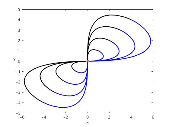
Consider a plane problem governed by the system of autonomous equations

\[ \dot{x} = x^2 -3\,xy, \qquad \dot{y} = 2xy-y^2 . \]
To generate plots of solutions, we numerically solve the autonomous system subject some initial conditions. Then we plot solutions on some finite time interval. While the paramter, which we usually denote by \( t ,\) corresponds to the infinite parameter interval \( -\infty < t< \infty \) with the point \( (x(t), y(t) ) \) on the trajectory approaching the origin as \( t \mapsto \pm \infty \) , but the finite interval \( -10 < y <10 \) suffices for graphical purposes.


function project
for n = -4:4
    [~,sol]=ode45(@diffeq,[0,10],[n,n]);
    plot(sol(:,1),sol(:,2),'k','LineWidth',2)
    hold on
    [~,solu]=ode45(@diffeq,[0,-10],[n,n]);
    plot(solu(:,1),solu(:,2),'b','LineWidth',2)
    if n==0
       plot(solu(:,1),solu(:,2),'r*')
    end
end
    xlabel('x','FontSize',12);
    ylabel('y','FontSize',12,'Rotation',0);

  function dwdt = diffeq(~,w)
%   x' = x^2 -3xy
%   y' = 2xy -y^2
    x = w(1);
    y = w(2);
    dxdt = x^2 - 3*x*y;
    dydt = 2*x*y - y^2;
    dwdt = [dxdt;dydt];
  end
end
Linearization

Enter text here

Euler Systems of Equations
Conservative Systems
Lyapunov's Second Method
Linear and Bernoulli equations
Periodic Solutions
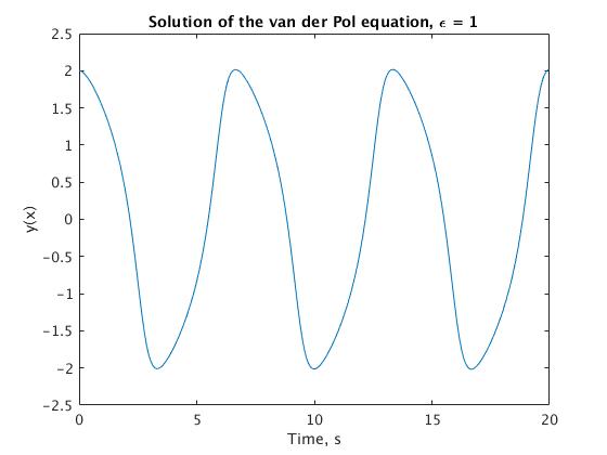
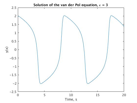
Van der Pol Equation
Relaxation oscillations are commonly associated with the name of Balthazar van der Pol (1889--1959) via his eponymous paper (Philosophical Magazine, 1926) in which he apparently introduced this terminology to describe the nonlinear oscillations produced by self-sustained oscillating systems such as a triode circuit. He modeled the oscillator with the following second order differential equation:
\[ \ddot{x} +\epsilon \left( x^2 -1 \right) \dot{x} + x =0, \]
where \( \epsilon \) is a positive parameter. While this differential equation was introduced by Lord Rayleigh in 1883, it was the Dutch electrical engineer and physicist van der Pol who investigated the corresponding oscillator extensively in 1920's and 1930's. Since then thousands of papers have been published achieving better approximations to the solutions occurring in such non linear systems. The van der Pol oscillator is a classical example of self-oscillatory system and is now considered as very useful mathematical model that can be used in much more complicated and modified systems.
function vanderpol
  xstart = 0; % Start value for x
  xstop = 20; % Terminal value for x
  yinitial = [2;0]; % Initial conditions

% Defining epsilon as a positive parameter
  for epsilon = 1:2:5
%   Solving van der Pol differential equations using ode45
    [xval,yval] = ode45(@differentialeqn,[xstart,xstop],yinitial);
    %Plot
    figure;
    plot(xval,yval(:,1));
    title(['Solution of the van der Pol equation, ','\epsilon = ',num2str(epsilon)]);
    xlabel('Time, s');
    ylabel('y(x)');
  end

function dydt = differentialeqn(~,y)
%   Vector-function that defines the van der Pol differential equation as
%   normal system of first order differential equations
    y1 = y(1);
    y2 = y(2);
    dy1dt = y2;
    dy2dt = epsilon*(1-(y1^2))*y2-y1;
%   Creates a vector that corresponds to derivatives
    dydt = [dy1dt;dy2dt];
  end
end
     
The relaxation oscillations have become the cornerstone of geometric singular perturbation theory and play a significant role in the analysis presented here. Van der Pol went on to propose a version of the above van der Pol equation that includes a periodic forcing term:
\[ \ddot{x} +\epsilon \left( x^2 -1 \right) \dot{x} + x = A\,\sin (\omega t) . \]

In a similar equation, he and van der Mark first noted the existence of two stable periodic solutions with different periods for a particular value of the parameters and observed noisy behavior in an electrical circuit modelled with the periodic driven term. Van der Pol and van der Mark in their investigations of the oscillator behaviour in the relaxation oscillation regime found that the subharmonical oscillations are appeared during changes of natural frequency of the system. Moreover, the authors (in the September 1927 issue of the British journal Nature), noted appearing of “irregular noise” before transition from one subharmonical regime to another. It seems to be it was one of the first observations of chaotic oscillations in the electronic tube circuit. Their paper is probably one of the first experimental reports of chaos – something that they failed to pursue in more detail.

Since its introduction in the 1920's, the van der Pol equation has been a prototype for systems with self-excited limit cycle oscillations. The classical experimental setup of the system is the oscillator with vacuum triode. The investigations of the forced van der Pol oscillator behaviour have carried out by many researchers. The equation has been studied over wide parameter regimes, from perturbations of harmonic motion to relaxation oscillations. It was much attention dedicated to investigations of the peculiarities of the Van der Pol oscillator behaviour under external periodic (sinusoidal) force and, in particular, the synchronization phenomena and the dynamical chaos appearing. The van der Pol equation is now concerned as a basic model for oscillatory processes in physics, electronics, biology, neurology, sociology and economics. Van der Pol himself built a number of electronic circuit models of the human heart to study the range of stability of heart dynamics. His investigations with adding an external driving signal were analogous to the situation in which a real heart is driven by a pacemaker. He was interested in finding out, using his entrainment work, how to stabilize a heart's irregular beating or "arrhythmias". Since then it has been used by scientists to model a variety of physical and biological phenomena. For instance, in biology, the van der Pol equation has been used as the basis of a model of coupled neurons in the gastric mill circuit of the stomatogastric ganglion. The Fitzhugh–Nagumo equation is a planar vector field that extends the van der Pol equation as a model for action potentials of neurons. In seismology, the van der Pol equation has been used in the development a model of the interaction of two plates in a geological fault.


Applications

Example 2.3.1: Quadcopter

Suppose that you want to investigate the performance of a feedback controller that is intended to hold a quadcopter at a prescribed altitude \( h. \) We assume that the quadcopter moves only vertically. Magnitude of the lift force (which comes from four engines, in newtons) is given by \( F_L = 4\,P(t)/ \left( \frac{v_y}{2} + \sqrt{\frac{mg}{\pi \rho L ^2}} \right) ; \) the power function is sum of three components: \( P(t)=k_p \,e(t)+k_d \, {\text d}e/{\text d}t+k_i\, \int e(t)\,{\text d}t \) . Thus, the error deviation from attitude \( h \) is \( e(t)= h-y, \quad {\text d}e/{\text d}t = {\text d}h/{\text d}t -{\text d}y/{\text d}t = -{\text d}y/{\text d}t \) because \( h \) is a constant; integral of \( e(t) \) we denote by \( Q, \) so \( Q (t) = \int e(t)\,{\text d}t \) and \( e(t)= {\text d}Q/{\text d}t =h-y . \)
Magnitude of the drag force is modeled by \( F_d =c\,v^2 .\) Here \( k_p , \ k_d , \) and \( k_i \) are 3 constants that can be tuned to give the best performance of the system. We use the following notations:
\( t \)
is time (in seconds);
\( v_y \) is vertical speed (meters per second) of vehicle;
\( L \)
is length of rotor blades (in meters);
\( \rho = 1.2 \,\mbox{kg/m}^2\)
-- air density;
\( P(t) = k_p \,e(t) + k_d \,\frac{{\text d}\,e}{{\text d}\,t} + k_i \,\int e(t)\,{\text d}t \)
is power (in watts) of one of four motors;
\( k_p, \ k_d , \ k_i \)
-- constants;
\( F_d = c\, v^2 \)
is drag force (in newtons), where c is a constant;
\( e= h-y \) is an error;
\( h \)
is an altitude.


So basically engine power \( P(t) \) is input, and \( h \) is a given attitude. Now we write the system of differential equations:

\[ \begin{split} \frac{{\text d}y}{{\text d} t} &= v_y , \\ \frac{{\text d} v_y}{{\text d} t} &= \frac{8\,P}{\left( v_y m +C \right)} - \frac{c\,v_y^2}{m} -g , \\ \frac{{\text d}Q}{{\text d} t} &= h-y , \end{split} \]
where \( C = 2m \,\sqrt{\frac{mg}{\pi \rho L^2}} . \) To solve this system of equations, we introduce the vector of three unknowns: \( {\bf w} = \langle y, v_y , Q \rangle^T \) (T stands for transposition). Then its derivative is

\[ \frac{{\text d}{\bf w}}{{\text d} t} = \left[ \begin{array}{c} {\text d}y/{\text d}t \\ {\text d}v_y /{\text d}t \\ {\text d}Q /{\text d}t \end{array} \right] = \frac{{\text d}}{{\text d} t} \left[ \begin{array}{c} y \\ v_y \\ Q \end{array} \right] , \]

which we denote as dwdt in Matlab code. We solve this system of equations numerically using the following numerical values:

	function helicopter
clear all;
% Below are the given constants
m=10/1000;% mass is actually 10 grams
L=2/100;  % length of the rotor blades in cm
c=0.0012; % constant number
p=1.2;    % air density in kg/m^3
g=9.8;    % gravity acceleration in m/sec^2
dhdt=0;   % fixed altitude
h=1;      % height
initial_condition1=[0;0;0]; %y=vy=Q=0

% write ode45 functions and plot
% under 1st set of Kp, Kd, Ki constants
Kp=1; Kd=0; Ki=0; % chosen Kp, Kd, Ki constants
[times_1,sols_1] = ode45(@helicopter, [0:0.1:20], initial_condition1);
figure
hold on
plot(times_1,sols_1(:,1),'LineWidth',2,'Color',[1,0,0])
ylabel('h (m)','Fontsize',16);
xlabel('time (s)','Fontsize',16);
title(('Height of Helicopter'),'Fontsize',20);

% under 2nd set of Kp, Kd, Ki constants
initial_condition2=[0;0;0];
Kp=1; Kd=0.2; Ki=0;
[times_2,sols_2] = ode45(@helicopter, [0:0.1:20], initial_condition2);
plot(times_2,sols_2(:,1),'LineWidth',2,'Color',[0,1,0])

% under 3rd set of Kp, Kd, Ki constants
initial_condition3=[0;0;0];
Kp=1; Kd=0.2; Ki=0.2;
[times_3,sols_3] = ode45(@helicopter, [0:0.1:20], initial_condition3);
plot(times_3,sols_3(:,1),'LineWidth',2,'Color',[0,0,1])
legend('K parameters1','K parameters2','K parameters3')

%solve for the height of the helicopter given different parameters and test
%the performance of the controller
    function dwdt = helicopter(t,w)
        y = w(1); vy=w(2); Q=w(3);
        dydt=vy; %vertical speed
        dvydt=8*(Kp*(h-y)+Kd*(dhdt-dydt)+Ki*Q)/(vy*m+2*m*sqrt(m*g/(pi*p*L^2)))-(c*vy^2/m)-g; %plug P(t) into FL
        dQdt=h-y; %accounts for error
        dwdt=[dydt;dvydt;dQdt];
end
end			
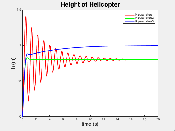
 

In the problem, the unknown functions \( y, \ v_y , \ Q \) are denoted by \( w(1), \,w(2), \, w(3) ,\) respectively. From the graph, we see that the third set of parameters \( k_p ,\, k_d , \,k_i \) controls the system with greater precision.

Example 2.3.2: Spacecraft

The lending motion of a spacecraft is modeled by the following system of differential equations

\[ \begin{split} \frac{{\text d}R}{{\text d}t} &= v_r , \\ \frac{{\text d}\theta}{{\text d}t} &= \omega , \\ \frac{{\text d}v_r}{{\text d}t} &= -B + R\,\omega^2 -C\,v_r , \\ \frac{{\text d}\omega}{{\text d}t} &= - \frac{2\,v_r \omega}{R} - C\,\omega , \end{split} \]
where
\[ B= g\,\frac{R^2_e}{R^2} , \qquad C= \frac{1}{2m}\, \rho_0 C_d \,A\,v_r \,e^{\left( -\frac{R-R_e}{d} \right)} , \qquad v= \sqrt{v_r^2 + \left( R\omega \right)^2} . \]
Here
\( \rho = \rho_0 \,e^{-h/d} \) is air density;
\( {\bf F}_d = - \frac{1}{2}\,\rho\,C_d A\,v\,{\bf v} \) is drag force,
\( v = \sqrt{v_r^2 + (R\omega )^2} \) is speed,
\( A \) is area of front,
\( C_d \) is drag coefficient,
\( {\bf F}_g = -mg\,\frac{R_e^2}{R^2}\,{\bf r} \) is gravitational force,
h is the distance above earth,
\( R \) is magnitude of position vector {\bf R},
\( R_e \) is radius of the earth.
We denote the unknow functions as \( R= w(1), \ \theta = w(2), \ v_r = w(3) .\) The initial conditions are as follows:
\( R= R_e + h_0 ,\)
\( \theta_0 =0 ,\)
\( v_r = v_0 \sin \phi , \)
\( \omega = v_0 \cos \phi /R ;\)
here \( \phi \) is re-entry angle, \( h_0 = 122\,\mbox{km} \) is the re-entry altitude. It is convenient to introduce the polar coordinates:
\[ x= R\,\cos\theta , \qquad y=R\,\sin\theta . \]


function capsule ??? to be modified
%% Problem 2
% We want to compute the trajectory of a spacecraft during reentry into the
% earth's atmosphere. Air density is given by p = po*e^(-h/d). Drag force
% is given by Fd = -1/2p*Cd*A*V. The gravitational force is given by Fg =
% -m*g*(Re^2/R^3). Use differential equations to relate R and theta and
% their time derivatives and solve for the trajectory of the spacecraft.

% Declare constants
m=8600;       % capsule mass in kg
A=2.5^2*pi;   % diameter of heat shield pi*r^2 in meters
Cd=0;         % drag coefficient
Re=6371*1000; % earth radius in m
d=5*1000;     % density decay length in m
p0=1.2;       % air density at sea level in kg/hr
h0=122*1000;  % re-entry altitude in meters
V0=32000*(1000/3600); % velocity at re-entry
g=9.8;        % gravity acceleration
phi=0;        % re-entry angle
options = odeset('Event',@event_function2,'RelTol',0.000001);
initial_condition = [Re+h0; 0; -V0*sin(phi); V0*cos(phi)/(Re+h0)]; %provide initial conditions
[times,sols] = ode45(@spacecraft,[0,(240*60)],initial_condition,options);

% write function to solve the trajectory of the spacecraft
    function dwdt = spacecraft(t,w)
        R = w(1); theta=w(2); vR=w(3); omega= w(4);
        v=sqrt(vR^2+(R*omega)^2);
        dRdt = vR;  dthetadt=omega;
        dvRdt = -g*(Re^2/R^2) + R*(omega^2) - (((1/2)*p0*Cd*A*v)/m)*exp(-(R-Re)/d)*vR;
        domegadt = (-(2*vR*omega)/(R))-((1/2)*(p0*Cd*A*v/m)*exp(-(R-Re)/d))*omega;
        dwdt = [dRdt;dthetadt;dvRdt;domegadt];
end
 function [val,stop,dir] = event_function2(t,w)
        R = w(1); theta=w(2); vR=w(3); omega = w(4);
        val = R-Re;
        stop = 1;   % this stops matlab when the spacecraft hits the ground
        dir = -1; % interested in y crossing zero from positive to negative
 end

for i=1:length(times)
    x(i) = sols(i,1)*cos(sols(i,2));
    y(i) = sols(i,1)*sin(sols(i,2));
end
% plot the spacecraft's trajectory
figure
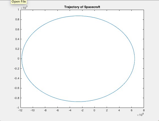
plot(x,y)
title('Trajectory of Spacecraft')
end			
 

Example 2.3.3: Lorenz Attractor

We will wrap up this series of examples with a look at the fascinating Lorenz Attractor. The Lorenz system is a system of ordinary differential equations (the Lorenz equations, note it is not Lorentz) first studied by the professor of MIT Edward Lorenz (1917--2008) in 1963. It is notable for having chaotic solutions for certain parameter values and initial conditions. In particular, the Lorenz attractor is a set of chaotic solutions of the Lorenz system which, when plotted,
\[ \begin{split} \frac{{\text d}x}{{\text d}t} &= \sigma\left( y-x \right) , \\ \frac{{\text d}y}{{\text d}t} &= x \left( \rho -z \right) -y, \\ \frac{{\text d}z}{{\text d}t} &= x\, y - \beta \, z . \end{split} \]

The equations are made up of three populations: x, y, and z, and three fixed coefficients: \( \sigma ,\ \rho , \mbox{ and } \ \beta .\) Remembering what we discussed previously, this system of equations has properties common to most other complex systems, such as lasers, dynamos, thermosyphons, brushless DC motors, electric circuits, and chemical reactions. First, it is non-linear in two places: the second equation has a xz term and the third equation has a xy term. It is made up of a very few simple components. The system is three-dimensional and deterministic. Although difficult to see until we plot the solution, the equation displays broken symmetry on multiple scales. Because the equation is autonomous (no t term in the right side of the equations), there is no feedback in this case.


This system’s behavior depends on the three constant values chosen for the coefficients. It has been shown that the Lorenz System exhibits complex behavior when the coefficients have the following specific values: \( \sigma = 10, \ \rho = 28 , \mbox{ and }\ \beta = 8/3. \) We now have everything we need to code up the ODE into Matlab. However, we will write two codes, one we call attractor.m, and another one is lorenz.m. We now have everything we need to code up the ODE into Matlab.
function attractor
% The Lorenz strange attractor
% Implements the Lorenz System ODE
%   dx/dt = sigma*(y-x)
%   dy/dt = x*(rho-z)-y
%   dz/dt = xy-beta*z%
% Inputs:
%   ~ - time variable: the name is not used here because system is autonomous.
%   Y - dependent variable: has 3 dimensions
% Output:
%   dYdt - First derivative: the rate of change of the three dimension
%        values over time, given the values of each dimension
t0=0; % Initial point
tn=20; % Terminal point
Y0=[10, 10, 10]; % Initial values
% Standard constants for the Lorenz Strange Attractor
sigma = 10;
rho = 28;
beta = 8/3;
[t, Y] = ode45(@ lorenz, [t0, tn], Y0); % RelTol 1e-3 (default)
% Create 3d Plot
figure('name','The Lorenz strange attractor')
plot3(Y(:,1), Y(:,2), Y(:,3));
grid
[t1,Y1] = ode45(@ lorenz, [t0, tn], Y0, odeset('RelTol', 1e-6));
figure('Name','The Lorenz strange attractor, comparison')
plot3(Y(:,1),Y(:,2),Y(:,3), Y1(:,1),Y1(:,2),Y1(:,3))
legend('RelTol 1e-3','RelTol 1e-6')
grid
figure('Name',...
  'The Lorenz strange attractor, RelTol 1e-3 (blue) and 1e-6 (red)')
subplot(3, 1, 1)
plot(t,Y(:,1), t1,Y1(:,1))
ylabel('x')
subplot(3, 1, 2)
plot(t,Y(:,2),t1,Y1(:,2))
ylabel('y')
subplot(3, 1, 3)
plot(t,Y(:,3), t1,Y1(:,3))
ylabel('z')
xlabel('t')
disp('Numbers of steps for RelTol 1e-3 and 1e-6')
disp([numel(t),numel(t1)])

  function dYdt = lorenz(~,X)
    % The Lorenz strange attractor
    dxdt = sigma*(X(2)-X(1));
    dydt = X(1)*(rho-X(3))-X(2);
    dzdt = X(1)*X(2)-beta*X(3);
    dYdt = [dxdt; dydt; dzdt];
  end
end

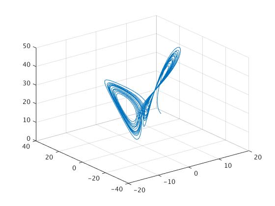
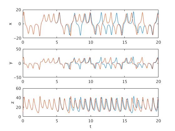
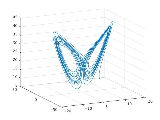
The output consists of the following graphs:

   
and three solutions for \( x(t),\ y(t) \) , and \( z(t) \) , respectively:

Matlab allow you to rotate the picture: just click on the icon and drag the cursor. You will get another view of the pictures:  


I have picked a starting point of [10 10 10] and I encourage you to play around with other starting points. Because this is a system of three equations, the solution can be plotted in three dimensions. Because the shape of the solution is somewhat complex, we can use “rotation” icon of tool bar and rotate 3D plot.

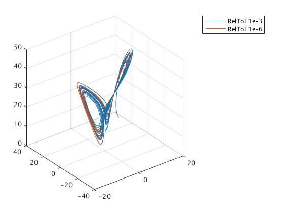
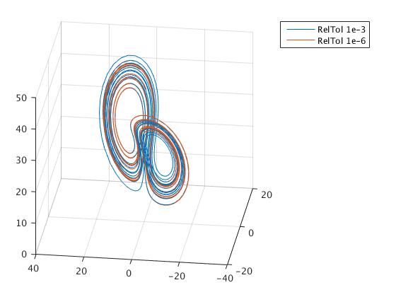
It turns out that Matlab allows you to choose how forgiving you want your solver to be. You can set the relative error tolerance (‘RelTol’) and the absolute error tolerance (‘AbsTol’). I simply changed the relative error tolerance. The default relative error tolerance is 0.001. I lowered a value of that tolerance down to 1e-6 (it means did a tolerance higher) and compared the two solutions. In the following examples, the red solution is generated using the 1e-6 relative tolerance. We set the error tolerance using the odeset function. Then we evaluate the solutions while passing in the returned value from the odeset function. Make note that in this example, the two solutions are using the exact same set of equations and starting at the exact same point.

As you can see, the two solutions do seem to diverge. You can see it somewhat clearly in the inner part of the orbits, where one shows mostly blue and the other red. Still, it’s tricky to see exactly how quickly and where the two diverge. To get a better look at it, we splitted the 3D graph into three separate graphs, one for each dimension. 

Keep in mind that this is the exact same graph as the previous figure, just plotted differently. Here we can indeed see that the two solutions diverge very rapidly (although rapidly may be a misnomer as we are ignoring units in this lesson). Blue and red seem to diverge somewhere between time 5 and 10, and while they do come back into close proximity, they never join back together (just like our logistic map example).

How did this difference happen? Recall what I said about how a higher error tolerance forces the numerical solver to take smaller steps. In each case, the solver went from time 0 to time 20. But, let’s see how many steps each took to get there. We printed these quantities

>> attractor
Numbers of steps for RelTol 1e-3 and 1e-6
        1233        4389


Thus, the same solver, solving the same equation, starting at the same starting point, took over 3.5 times more steps than the default approach when using a higher error tolerance. Furthermore, not only did it take more steps and presumably generate a more accurate solution, after a short period of similarity, the more accurate solver generated a completely different solution than the default solver! The interesting question is to ask, how quickly did our `good’ solver diverge from the real solution? It should be to always question the results of your numerical solutions to ODEs that describe complex and/or chaotic systems. It only takes small missteps for your solution to rapidly diverge from the actual solution.

We present another version solving Lorenz equations numerically and plotting the results. This includes several steps.

Step 1. Define an anonymous function, or save it as a separate function file. We write three dots in order to prolong the command.

mylorenz = @(x,sigma,rho,beta)...
[ sigma * (x(2) - x(1)); ...
rho * x(1)-x(1) * x(3) - x(2); ...
x(1) * x(2) - beta * x(3) ];
Step 2. Specify the parameters and define an anonymous function that can be used by an ODE solver.
sigma = 10; beta = 8/3; rho = 30;
lorenzxdot = @(t,x) mylorenz(x,sigma,rho,beta);

Note:These two lines above need to be run each time when any of the parameters is changed.

Step 3. Choose initial values and a time interval for the solution and compute an approximate using a built-in Runge–Kutta solver.

x0 = [3;4;1];
Tmax = 40;
[time,solvec] = ode45(lorenzxdot, [0,Tmax],x0);

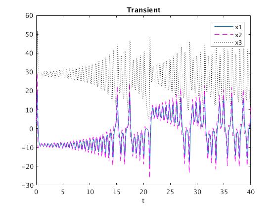
The solutions can then be plotted next to each other or in a three-dimensional plot.

figure
plot(time,solvec(:,1),'-',time,solvec(:,2),'m--',time,solvec(:,3),'k:')
legend('x1','x2','x3')
title('Transient')
xlabel('t')
% Will plot x(1) and x(2) as a function of time on the same graph.
figure
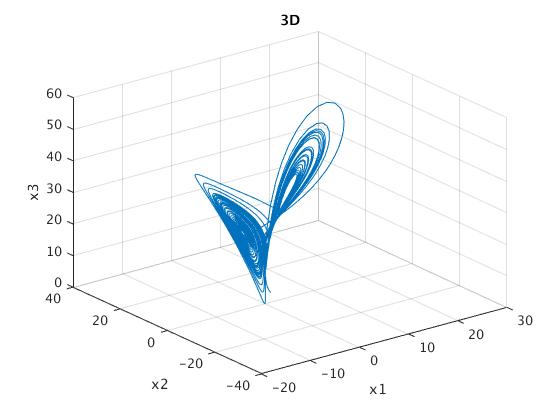
plot3(solvec(:,1),solvec(:,2),solvec(:,3))
xlabel('x1')
ylabel('x2')
zlabel('x3')
title('3D')
grid on
   
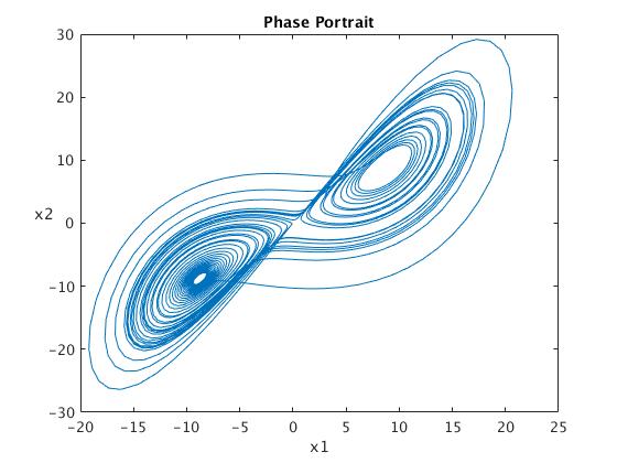
While the following will be a plot in the phase plane for x(1) and x(2):
figure
plot(solvec(:,1),solvec(:,2))
xlabel('x1')
ylabel('x2','rotation',0)
title('Phase Portrait')
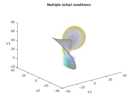
% Multiple Initial Conditions
x1_0 = -5:2:5;
y1_0 = -5:2:5;
z1_0 = -10:2:10;
Tmax = 10;
figure
view(3);
title('Multiple initial conditions')
xlabel('x1')
ylabel('x2')
zlabel('x3','rotation',0)
hold on
for i = 1:numel(x1_0)
  for j = 1:numel(y1_0)
    for k = 1:numel(z1_0)
      x0 = [x1_0(i);y1_0(j);z1_0(k)];
      [time,solvec] = ode45(lorenzxdot, [0,Tmax],x0);
      plot3(solvec(:,1),solvec(:,2),solvec(:,3),'Color',...
        [(-min(x1_0) + i)/(2*numel(x1_0)), (-min(y1_0) +j)/...
        (2*numel(y1_0)), (-min(z1_0) + k)/(2*numel(z1_0))]) %fun colors
      drawnow
    end
  end
end
hold off
   
Ensemble
In order to simulate the Lorenz equations for an ensemble of initial data, define the functions mylorenz and lorenzxdot as above, together with suitable choices for the parameters sigma, beta, rho. Let Tmax be the length of the time interval, and let N be the ensemble size (the number of simulations). The following code computes the means of N with initial data x0 + xi , where xi is a normal random vector with zero mean and standard deviation gamma.
N = 10;
gamma = .5;
Tmax = 40;
x0 = [3;15;1];
tt = linspace(0,Tmax,10*Tmax);
xEns = 0*tt;
yEns = 0*tt;
zEns = 0*tt;
for j = 1:N
[t,solvec] = ode45(lorenzxdot, [0,Tmax],x0 + gamma*randn(3,1));
% tt corresponds to the points of interpolation;
xEns = xEns + spline(t,solvec(:,1),tt);
yEns = yEns + spline(t,solvec(:,2),tt);
zEns = zEns + spline(t,solvec(:,3),tt);
end
xEns = xEns/N;
yEns = yEns/N;
zEns = zEns/N;

figure
plot(tt,xEns,'r',tt,yEns,'g',tt,zEns,'b')
legend('xEns','yEns','zEns')
title('Ensemble')
xlabel('t')
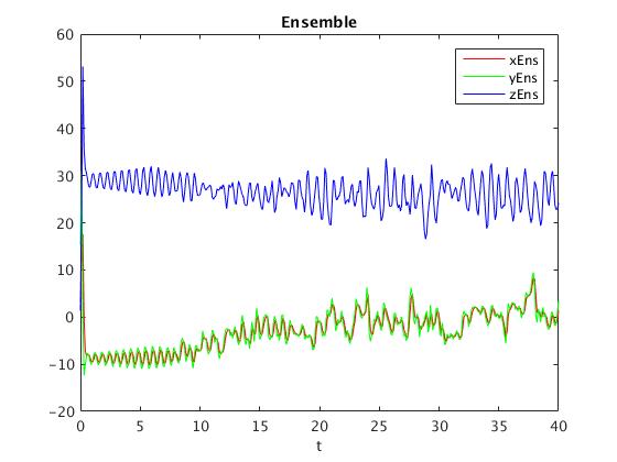
We use spline command (which is actually cubic interpolation) because the standard procedure ode45 for solving differential equations numerically is based on Runge--Kutta method with variable steps. This part of code can be replaced with linear interpolation:

xEns = xEns + interp1(t,solvec(:,1),tt);
yEns = yEns + interp1(t,solvec(:,2),tt);
zEns = zEns + interp1(t,solvec(:,3),tt);				

In dynamical systems, a first recurrence map or Poincaré map, named after Henri Poincaré, is the intersection of a periodic orbit in the state space of a continuous dynamical system with a certain lower-dimensional subspace, called the Poincaré section, transversal to the flow of the system. More precisely, one considers a periodic orbit with initial conditions within a section of the space, which leaves that section afterwards, and observes the point at which this orbit first returns to the section. One then creates a map to send the first point to the second, hence the name first recurrence map. The transversality of the Poincaré section means that periodic orbits starting on the subspace flow through it and not parallel to it. A Poincaré map can be interpreted as a discrete dynamical system with a state space that is one dimension smaller than the original continuous dynamical system. Because it preserves many properties of periodic and quasiperiodic orbits of the original system and has a lower-dimensional state space, it is often used for analyzing the original system in a simpler way. In practice this is not always possible as there is no general method to construct a Poincaré map.

In the Poincaré section method one records the coordinates of a trajectory whenever the trajectory crosses a prescribed trigger. This triggering event can be as simple as vanishing of one of the coordinates, or as compli cated as the trajectory cutting through a curved hypersurface. A Poincaré section (or, in the remainder of this chapter, just ‘section’) is not a projection onto a lower-dimensional space: rather, it is a local change of coordinates to a direction alo ng the flow, and the remaining coordinates (spanning the section) transverse to it. No information about the flow is lost by reducing it to its set of Poincaré section points and the return maps connecting them; the full space trajectory can a lways be reconstructed by integration from the nearest point in the section.


Reduction of a continuous time flow to its Poincaré section is a powerful visualization tool. But, the method of sections is more than vi sualization; it is also a fundamental tool of dynamics - to fully unravel the geometry of a chaotic flow, one has to quotient all of its symmetries
Pendulum Equations
Population Models
Let’s look at one more example. An SIR model is an epidemiological example of an infection invading a population. In the beginning most people are healthy and the infection spreads slowly. As more people get sick, the infection begins to grow noticeably. Eventually, the population begins to recover and gains an immunity to the infection. Thus, the susceptible population disappears and is replaced by a resistant population. The three populations modeled in the standard SIR equation are susceptible, infected, and recovered.
\[ \begin{split} \frac{{\text d}S}{{\text d}t} &= -\beta\, S\,I , \\ \frac{{\text d}I}{{\text d}t} &= \beta\, S\,I - \delta \,I, \\ \frac{{\text d}R}{{\text d}t} &= \delta\, I . \end{split} \]

The first thing to note is that there are only two terms. The first, \( \beta \,S\,I \) describes the rate of infection. This term scales positively with both the susceptible population and the infected population. The more people susceptible, the easier it is to find a new host. The more infected people, the more there are to spread the disease. Also note that the exact same quantity that is removed from the susceptible population is added to the infected population. This represents a direct state transition from one population to the other. Similarly, as infected people gradually recover at a rate \( \delta \,I , \) they are removed from the infected population and added to the recovered population. Finally, note that if you add all three equations together you get a net effect of \( \left( {\text d}S+{\text d}I+{\text d}R\right) /{\text d}t = 0. \) This shows that the total population is stable: there is no addition or removal of people, only changes in their state.


Let’s code this up! First, the function definition (I will set the constants to be \( \beta = .003 \) and \( \delta = 1: \)

% sir.m
%
% Imlements a SIR infection model
%   dS/dt = -beta SI
%   dI/dt = beta SI - delta I
%   dR/dt = delta I
%
% Inputs:
%   t - Time variable: not used here because our equation
%       is independent of time, or 'autonomous'.
%   x - Independent variable: this contains three
%       populations (S, I, and R)
% Output:
%   dx - First derivative: the rate of change of the populations
function dx = sir(t, x)
  dx = [0; 0; 0];
  beta = .003;
  delta = 1;

  dx(1) = -beta * x(1) * x(2);
  dx(2) = beta * x(1) * x(2) - delta * x(2);
  dx(3) = delta * x(2);				
We will use the same options, but add one extra non-negative population (as we now have three).
options = odeset('RelTol', 1e-4, 'NonNegative', [1 2 3]);
Finally, we will model an infection of a population of 1000 healthy individuals and 1 sick person. The time interval will go from 0 to a unitless 10.
% Use ode45 to solve our ODE
% Place the time points in a vector 't'
% Place the solution in a vector 'x'
[t,x] = ode45('sir', [0 10], [1000 1 0], options);
plot(t,x);
legend('S', 'I', 'R');
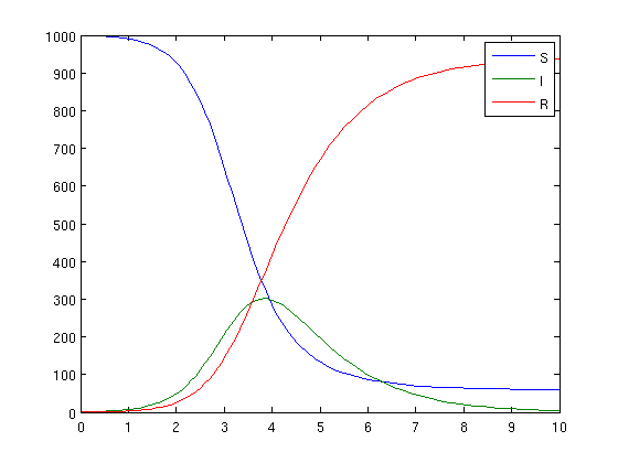
And here is our result:
Notice how the infection initially picks up steam and spreads quickly through the population but soon runs out of gas as the susceptible population quickly drops. The simulation will continue indefinitely as the infected population will slowly decay and the recovered population will asymptotically approach 1001.
Preditor-Prey Equations


Given that the Arctic ground squirrel (Spermophilus parryii) lives in the same ecosystem as the red fox (Vulpes vulpes), the fox population preys on the squirrel population. An ecologist wants to look at a population model for both the Arctic ground squirrel and the red fox in a region of the Denali National Park and Preserve in Alaska for the next fifteen years, given that there are currently 250 squirrels and 20 foxes in the specific region. A way to look at the population fluctuations of both populations over a period of time would be via the Lotka-Volterra model.

Let us start with a simple Lotka-Volterra predator/prey two-body simulation. There are two populations in question: the predators and the prey. Prey grow exponentially, when their is no constraint. However, prey are also killed off by the predators at a rate directly proportional to both the predator and prey population. Predators are dependent on prey for sustenance and thus grow at a rate dependent on both the predator and prey population. Predators also die off over time due to age. The Lotka-Volterra model assumes that the prey (squirrel) population’s growth is exponential and independent of the predator (fox) population, but the decline of the squirrel population is affected by both its own population size as well as the fox population size.

Another assumption is that the fox population is directly proportional to the squirrel population size as well as its own, but that the death rate of the fox population is independent of the squirrel population, since squirrels do not prey on foxes.

This gives us two populations each with two separate terms to add to our equation. Because both predator and prey start with ‘p’, we will use the variable x to refer to the prey population and the variable y to refer to the number of predators. Given that both x and y are functions of time, we have the following system of ODEs:

\[ \begin{split} \frac{{\text d}x}{{\text d}t} &= \alpha\, x - \beta\,x\,y , \\ \frac{{\text d}y}{{\text d}t} &= \delta\, x\,y - \gamma\,y . \end{split} \]

Let’s break things down. The top equation defines how the population of prey, x, changes in relation to the predator and prey populations. The first term, \( \alpha\, x ,\) is positive and therefore defines growth. The growth rate is proportional to x, so we know it is positive exponential growth (as seen in previous lessons). The \( \alpha \) term is a constant that controls how fast the exponential growth occurs. The second term, \( -\beta\, x\,y ,\) is negative and thus describes death. The rate is proportional to both x and y. This is because more prey makes it easier for predators to find prey and also because an increase in predators makes it harder for the prey to hide. In contrast, we assume an increase in predators does not affect the birth rate of the prey and thus there is no y in the growth term. Thus, \( \beta\, x\, y \) defines the rate at which predators find and kill prey, at an efficiency controlled by the constant \( \beta . \)

  The second equation defines the change in the predator population. The first term, δxy is positive and defines growth. Predators rely on prey for sustenance and thus grow proportionally to both their own population and the prey population at a rate controlled by \( \delta . \) For the second term, because prey can’t kill predators, the predator population only decays proportionally to their own numbers at a rate determined by \( \gamma . \)

It is important to note that both equations have an xy term. This means that both equations are non-linear and thus very difficult to deal with analytically. This is one of the reasons we will turn to numerical integration.


Now, let’s look at the expected dynamics before we actually plug in the equation. We have two populations, so let’s look at the different combinations of high and low populations of each. We want to pick coefficients such that the model is stable. If both populations are low, there needs to be positive growth to restore balance. This growth should come from the prey population being able to multiply without fear of many predators. Thus, the \( \alpha \) term must out-pace the \( \beta \) term for small values of x and y. If both values are high, there needs to be death to restore equilibrium. Thus the prey needs to die off due to a large predator population and the \( \beta \) term will dominate. If there is a lot of prey with few predators, the predator population should grow quickly. Conversely, if there are many predators and few prey, the predators population should diminish. If all of this happens, our system should be able to stay in some sort of periodic equilibrium. To this end, I will somewhat arbitrarily chose the constants to be: \( \alpha = 1,\ \beta = .05, \ \delta = .02, \ \mbox{ and } \ \gamma = .5. \)

  First, we will code up the equations as a Matlab function. Since we are dealing with two variables, our x parameter is now a vector containing both the prey and predator populations.

% lotka_volterra.m
%
% Imlements the Lotka-Volterra function
%   dx/dt = alpha x - beta xy
%   dy/dt = delta xy - gamma y
%
% Inputs:
%   t - Time variable: not used here because our equation
%       is independent of time, or 'autonomous'.
%   x - Independent variable: this contains both populations (x and y)
% Output:
%   dx - First derivative: the rate of change of the populations
function dx = lotka_volterra(t, x)
  dx = [0; 0];
  alpha = 1;
  beta = .08;
  delta = .02;
  gamma = .5;

  dx(1) = alpha * x(1) - beta * x(1) * x(2);				

Unless you plan on modifying your coefficients through external code it’s better to define them inside the function. Also note that x(1) refers to the prey and x(2) refers to predators.

Next, we need to use odeset to set our options. Note that now both populations 1 and 2 are non-negative.


% Set our preferences for ode45
% The default relative tolerance is 1e-3.
% To set our output to non-negative, we provide an array listing
%   each population that we want to constrain.  Since this example
%   has two populations, we pass the array [1 2]
options = odeset('RelTol', 1e-4, 'NonNegative', [1 2]);
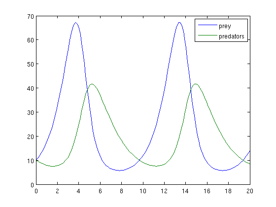
Finally, we use the ode45 function and plot out the results. We will initialize each population to 10 and will integrate from time 0 to 20. The time units here are completely arbitrary since we are using unitless coefficients.

% Use ode45 to solve our ODE
% Place the time points in a vector 't'
% Place the solution in a vector 'x'
[t,x] = ode45('lotka_volterra', [0 20], [10 10], options);
plot(t,x);
legend('prey', 'predators');
Which gives us a final result pictured here:
Notice the nice cyclical behavior. At first, prey multiply rapidly and predators decline a bit. As the prey population soars, predators find more food and begin to grow as well. Eventually the predators eat too many prey and lose numbers to starvation. This lets the prey rebound and the cycle begins again.