matlab provides many useful instructions for the visualization of 3D data. The instructions provided include tools to plot wire-frame objects, 3D plots, curves, surfaces, etc. and can automatically generate contours, display volumetric data, interpolate shading colors and even display non-Matlab made images.
| Order | Function |
| plot3(x,y,z,'line shape') | Space curve |
| meshgrid(x,y) | Mesh plot |
| mesh(x,y,z) | hollow mesh surface |
| surf(x,y,z) | mesh surface, solid filled |
| shading flat | flat/smooth surface space |
| countour3(x,y,z,n) | 3-dimensional equivipotential (n) lines |
| contour(x,y,z) | contours |
| meshc(x,y,z) | hollow grid graph projected by equivipotential lines |
| [x,y,z]=cylinder(r,n) | 3-dimensional curve surfaces |
We show how to use plotting commands by examples.
Example:
In the interval [0, 10*π], draw the parametric curve:
\( x = \sin (t), \ y = \cos (t), \ z = t. \)
We type in the following matlab code:
t=0:0.01:10*pi;
plot3(sin(t),cos(t),t)
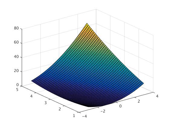
Example: Plot a surface \( z=(x+y)^2 \)
x=-3:0.1:3;
y=1:0.1:5;
[x,y]=meshgrid(x,y);
z=(x+y).^2;
plot3(x,y,z)
When using ''meshgrid,'' the coding should be changed into:
x=-3:0.1:3;
y=1:0.1:5;
[x,y]=meshgrid(x,y);
z=(x+y).^2;
mesh(x,y,z)
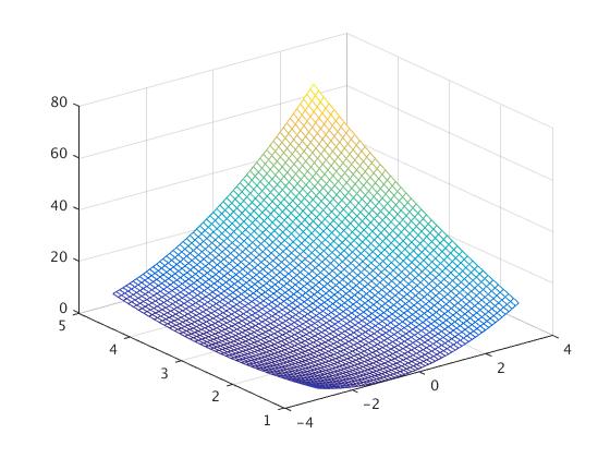
Or the solid filled:
x=-3:0.1:3;
y=1:0.1:5;
[x,y]=meshgrid(x,y);
z=(x+y).^2;
surf(x,y,z)
And with the flat surface:
x=-3:0.1:3;
y=1:0.1:5;
[x,y]=meshgrid(x,y);
z=(x+y).^2;
surf(x,y,z)
shading flat
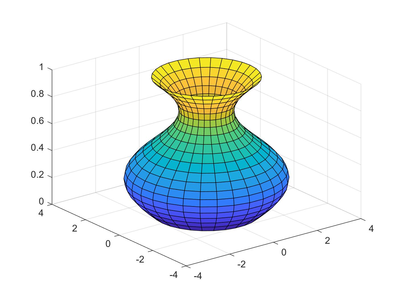
Example:
Consider a 3-dimensional rotating surface ([x,y,z]=cylinder(r,n))
We plot the 3D graph for \( r(t)=2+\sin (t)
. \)
Using “mesh, cylinder” the code will be as follows
t=0:pi/10:2*pi;
r=2+sin(t);
[x,y,z]=cylinder(r,30);
mesh(x,y,z)
with the Solid filled
t=0:pi/10:2*pi;
r=2+sin(t);
[x,y,z]=cylinder(r,30);
surf(x,y,z)
Or with the “shading flat”:
t=0:pi/10:2*pi;
r=2+sin(t);
[x,y,z]=cylinder(r,30);
surf(x,y,z)
shading flat
Now we plot the function of r(t)=2+sin(t), using the 3-dimension equipotential lines
t=0:pi/10:2*pi;
		  r=2+sin(t);
		  [x,y,z]=cylinder(r,30);
	    contour3(x,y,z,20)
Or:
t=0:pi/10:2*pi;
r=2+sin(t);
[x,y,z]=cylinder(r,30);
meshc(x,y,z)
Or:
t=0:pi/10:2*pi;
r=2+sin(t);
[x,y,z]=cylinder(r,30);
surfc(x,y,z)
■
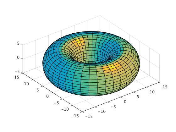
Example:
Toroid surface:
a=5; % a and c are arbitrary constants
c=10;
[u,v]=meshgrid(0:10:360); % meshgrid produces a full grid represented by the output coordinate arrays u and v; u and v are time variables
x=(c+a*cosd(v)).*cosd(u); % x, y, and z are the parameterized equations for a toroid
y=(c+a*cosd(v)).*sind(u);
z=a*sind(v);
surfl(x,y,z) % surfl creates a surface plot with colormap-based lighting
axis equal; % scales the axis so the x, y, and z axis are equal
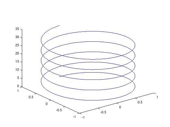
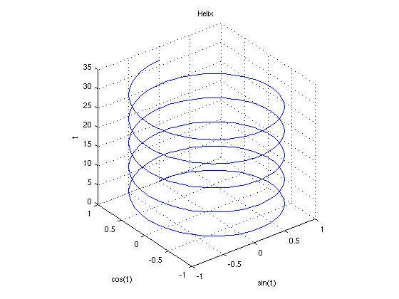
Example 0.1.4: Helix
t = 0:pi/50:10*pi; %create the vector t. starting value of 0, each element increases pi/50 from the previous up through 10*pi
plot3(sin(t),cos(t),t) %3D plot, coordinate (x, y, t)
title('Helix') %creates plot title
xlabel('sin(t)') %creates x label
ylabel('cos(t)') %creates y label
zlabel('t') %creates t label
grid on %dashed grids
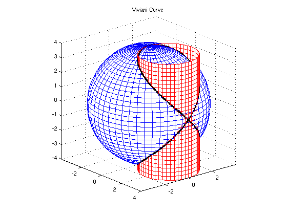
Example 0.1.5:
% The Viviani's Curve is the intersection of sphere x^2 + y^2 + z^2 = 4*a^2
%and cylinder (x-a)^2 +y^2 =a^2
%This script uses parametric equations for the Viviani's Curve,
%and the cylinder and sphere whose intersection forms the curve.
% For the sphere:
  a = 2; %the parameter 'a' from the equations, here a=2
  phi = linspace(0,pi,40); %this defines the scope of phi, from 0 to pi, the '40' indicates 40 increments between the bounds
  theta = linspace(0,2*pi,50); %this defines the scope of theta
  [phi,theta] = meshgrid(phi,theta); %creates a grid of (phi,theta) ordered pairs
  %the parametric equation for the sphere:
  x=2*a*sin(phi).*cos(theta); %use a '.' before the operator, this is an array operation
  y=2*a*sin(phi).*sin(theta); %the . indicates that this operation goes element by element
  z=2*a*cos(phi); %note: always suppress data using a semicolon


  %Plotting the sphere:
  mhndl1=mesh(x, y, z); %'mhndl' plots and stores a handle of the meshgrid
  set(mhndl1,... % formats 'mhndl'
  'EdgeColor',[0,0,1]) %gives the surface color, [0,0,1] is a color triple, vary the combination to get different color
  axis equal %controls axis equality, this is very important for ensuring the sphere looks perfectly round
  axis on %controls whether axes are 'on' or 'off'


%For the cylinder:
  t=linspace(0,2*pi,50); %defines the scope of 't'
  z=linspace(-2*a,2*a,30); %defines the scope of 'z', the bounds for the top and bottom of the cylinder
  [t,z]=meshgrid(t,z); %creates pairs of (t,z)
x=a+a*cos(t); %the parametrized cylinder
  y=a*sin(t);
  z = 1*z;
%Plotting the cylinder
  hold on %prevents override of plot data, so both the cylinder and sphere can occupy the same plot
  mhndl2=mesh(x, y, z); %notice 'mhndl' is numbered, mhndl2=mesh(x,y,z) plots the cylinder
  set(mhndl2,...
  'EdgeColor',[1,0,0]) %[1,0,0] gives the color red
  view(50,20)
%view(horizontal_rotation,vertical_elevation) sets the angle of view,
%both parameters used are measured in degrees


%For the actual Vivani's Curve:
  t=linspace(0,4*pi,200); %scope of the 't' values
  x= a+a*cos(t); %parametrized Viviani's Curve
  y= a*sin(t);
  z = 2*a*sin(t/2);
  %To plot the Viviani's Curve:
  vhndl = line( x,y,z); %here 'vhndl' is used to plot the curve and record the handle
  set(vhndl, ...
  'Color', [0,0,0],... % here [0,0,0] gives the color black
  'LineWidth',3) %line width of the line
  view(50,20);
%similar to before, this indicates 50 degrees horizontal rotation, 20 degrees vertical elevation


%Adding a title
  title('Viviani Curve') %to add a title, use title('Title')
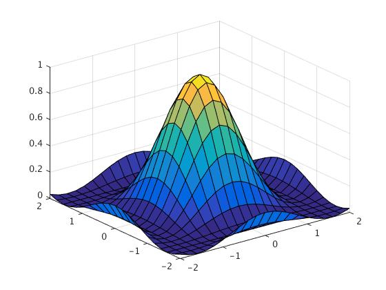
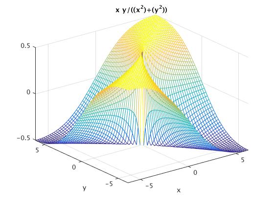
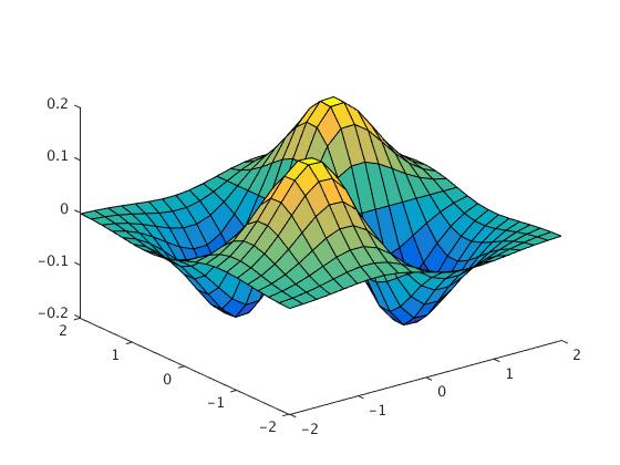
Example 0.1.6:
Some other simple 3D curves:
[x,y] = meshgrid(-2:0.2:2,-2:0.2:2);
z=x.*y.*exp(-x.^2-y.^2);
figure
surface(x,y,z)
view(3)
z=(cos(x).^2).*(cos(y).^2);
surf(x,y,z)