The Wolfram Mathematica notebook which contains the code that produces all the Mathematica output in this web page may be downloaded at this link.
$Post :=
If[MatrixQ[#1],
MatrixForm[#1], #1] & (* outputs matricies in MatrixForm*)
Remove[ "Global`*"] // Quiet (* remove all variables *)
The conjugate gradient method is a family of algorithms for numerical solutions of particular systems of linear equations A x = b with symmetric (or self-adjoint in case when A ∈ ℂn×n) positive definite matrix A. Its variation is known as the biconjugate gradient method and provides a generalization for solving equations with non-symmetric matrices (but it may suffer from numerical instability).
The conjugate gradient algorithm always converges to
the exact solution of A x = b in a finite number of iteration steps in infinite precision arithmetics (in the absence of roundoff errors). In this
sense it is not really an iterative method from mathematical prospective. It can be viewed as a “direct method” like
Gaussian elimination, in which a finite set of operations produces the exact solution.
However, there are several good reasons to interpret the conjugate gradient method as an iterative method rather than a direct method.
First of all, execution of this algorithm can be stopped partway at any stage, similar to any iterative method.
Despite that the conjugate gradient method uses memory of all previous steps---it can be organized in the form of one step iterative algorithm that generates a finite sequence of approximations
\begin{equation*}
{\bf x}^{(k)} = g_k \left( {\bf x}^{(k-1)} \right) , \qquad k = 1, 2, \ldots , m \leqslant n ,
\end{equation*}
that always converges (in infinite arithmetics) to the true solution x* of equation A x = b.
In finite precision arithmetic, the conjugate gradient method behaves similarly to any iterative method where difference between two successive iterates may be quite subtle.
In practice, the conjugate gradient method frequently “converges” to a sufficiently accurate approximation to x✶ in far less than n iterations (where n is the size of the problem).
The conjugate gradient method (henceforth, CG) was developed independently by the American mathematician
Magnus Hestenes (1906–1991) and Eduard Steifel (1907–1998)
from Switzerland in the early fifties. Later, they met during the "Symposium on Simultaneous
Linear Equations and the Determination of Eigenvalues," organized in Los Angeles in 1951
by the Institute of Numerical Analysis of the U.S. National Bureau of Standards. They realized that their algorithms were the same and wrote a famous joint paper that was published in 1952. About the same time, Cornelius Lanczos (1893--1974) invented a similar algorithm, but he applied it to eigenvalue problems.
Actually, the CG algorithm is a particular case of more general method known as the Krylov subspace iteration and it is the most famous of these methods because it is now the main algorithm for solving large sparse linear systems.
The latter approach was invented in 1931 by the Russian mathematician and naval engineer Alexey Krylov (1863--1945).
To solve an n × n positive definite linear system by a direct method and the CG algorithm,
requires n steps by both methods to determine a solution, and the steps of the conjugate gradient method are more
computationally expensive than those of Gaussian elimination.
However, the conjugate gradient method is useful for solving large sparse systems with nonzero entries occurring in
predictable patterns. When the matrix has been preconditioned
to make the calculations more effective, good results are obtained in only about √n iterations.
where x is an unknown column vector, b is a known column vector, and A is a known, square, symmetric, positive-definite matrix. As usual, we denote by ℂm×n or ℝm×n the set of all m-by-nmatrices with entries from the field of complex or real numbers, respectively. These systems arise in many important settings, such as finite difference and finite element
methods for solving partial differential equations, structural analysis, circuit analysis, and math homework.
Example 1:
We start with a one-dimensional version of Poisson's equation for Laplace's operator Δ,
\[
-\frac{{\text d}^2 u}{{\text d}x^2} = f(x) , \qquad 0 < x < \ell ,
\tag{1.1}
\]
where f(x) is a given function and u(x) is the unknown function that we want
to compute. Function u(x) must also satisfy the Dirichlet boundary conditionsu(0) = u(ℓ) = 0. Of course, other boundary conditions (such as Neumann or of the third kind) can be supplied to Laplace's operator; however, we choose one of possible simple conditions for our illustrative example.
Recall that a differential operator is called positive (or negative) if all its eigenvalues are positive (or negative, respectively). Since the second order derivative operator \( \displaystyle \quad \texttt{D}^2 = {\text d}^2 / {\text d}x^2 \quad \) is negative, it is customary to negate the Laplacian.
We discretize the boundary value problem by trying to compute an approximate solution at N + 2 evenly spaced points xi between 0 and ℓ: xi = i h, where h = ℓ/(N+1) and 0 ≤ i ≤ N + 1. We abbreviate ui = u(xi) and fi = f(xi). To convert differential equation (1.1) into a linear equation for the unknowns u₁, u₂, … , uN, we use finite differences to approximate
\[
\left. \frac{{\text d}u}{{\text d}x} \right\vert_{x = (i-1/2) h} \approx \frac{u_{i} - u_{i-1}}{h} ,
\]
\[
\left. \frac{{\text d}u}{{\text d}x} \right\vert_{x = (i+1/2) h} \approx \frac{u_{i+1} - u_{i}}{h} .
\]
Subtracting these approximations and dividing by h yields the centered
difference approximation
\[
\left. \frac{{\text d}^2 u}{{\text d}x^2} \right\vert_{x = i h} \approx \frac{2 u_i - u_{i-1} - u_{i+1}}{h^2} + \tau_i ,
\]
where τi, the so-called truncation error, can be shown to be \( \displaystyle \quad O\left( h^2 \cdot \left\| \frac{{\text d}^4 u}{{\text d}x^4} \right\|_{\infty} \right) . \quad \)
We may now rewrite equation (1.1) at x = xi as
\[
- u_{i-1} + 2\,u_i - u_{i+1} = h^2 f_i + h^2 \tau_i ,
\tag{1.2}
\]
where 0 < i < N + 1. From Dirichlet's boundary conditions, we derive that u₀ = uN+1 = 0. Hence, we get
N equations with N unknowns u₁, u₂, … , uN:
\[
{\bf T}_N {\bf u} = h^2 \begin{pmatrix} f_1 \\ \vdots \\ f_N \end{pmatrix} + h^2 \begin{bmatrix} \tau_1 \\ \vdots \\ \tau_N \end{bmatrix} ,
\]
where
\[
{\bf T}_N = \begin{bmatrix} 2 & -1 & 0 & \cdots & 0 \\ -1& 2 & -1 & \cdots &0 \\ \vdots & \vdots & \vdots & \ddots & \vdots \\ 0&0&0& \cdots & -1 \end{bmatrix} , \qquad {\bf u} = \begin{pmatrix} u_1 \\ \vdots \\ u_N \end{pmatrix} .
\tag{1.3}
\]
To solve this system of equations, we will ignore terms with τ because they are small compared to f. This yields
\[
{\bf T}_N {\bf v} = h^2 {\bf f} .
\]
The coefficient matrix TN plays a central role in all that follows, so we will
examine it in some detail. First, we will compute its eigenvalues and eigenvectors. One can easily use trigonometric identities to confirm the following
lemma.
Lemma:
The eigenvalues of TN are
\( \displaystyle \quad \lambda_j = 2 \left( 1 - \cos \frac{\pi j /\ell}{N+1} \right) . \quad \) The corresponding eigenvectors are
\[
z_j (k) = \sqrt{\frac{2}{N+1}}\,\sin \left( \frac{jk\pi /\ell}{N+1} \right) , \qquad \| z_j \|_2 = 1.
\]
Let Z = [ z₁, z₂, … , zN ] be the orthogonal matrix whose columns are the eigenvectors, and Λ = diag(λ₁,λ₂, … , λN), so we can write \( \displaystyle \quad {\bf T}_N = {\bf Z}\,\Lambda \,{\bf Z}^{\mathrm T} . \)
Hence, the largest eigenvalue is
\( \displaystyle \quad \lambda_N = 2 \left( 1 - \cos \frac{\pi/\ell}{N+1} \right) \quad \)
and the smallest eigenvalue is λ₁, where for small i,
\[
\lambda_i = 2 \left( 1 - \cos \frac{i\pi}{N+1} \right) \approx 2 \left( 1 - \left( 1 - \frac{i^2 \pi^2}{2 (N+1)^2} \right) \right) = \left( \frac{i\pi}{N+1} \right)^2 .
\]
Therefore, matrix TN is symmetric and positive definite with condition number \( \displaystyle \quad \lambda_N / \lambda_1 \approx \frac{4}{\pi^2} \left( N+1 \right)^2 \quad \) for large N. The eigenvectors are sinusoids with lowest frequency at j = 1 and
highest at j = N.
Now we know enough to bound the error, i.e., the difference between the
solution of \( \displaystyle \quad {\bf T}_N \hat{\bf u} = h^2 {\bf f} \quad \) and the true solution u of the Dirichlet boundary value problem. Taking norms, we get
\[
\| u - \hat{u} \|_2 \le h^2 \| {\bf T}_N^{-1} \|2 \| \tau \|_2 \approx h^2 \left( \frac{N+1}{\pi} \right)^2 \| \tau \|_2 ,
\]
which has an order of
\[
O \left( \| \tau \|_2 \right) = O \left( h^2 \left\| \frac{{\text d}^4 u}{{\text d} x^4} \right\|_{\infty} \right) .
\]
Hence, the error \( \displaystyle \quad u - \hat{u} \quad \) goes to zero proportionally to h², provided that the solution is smooth enough (its fourth derivative is bounded on the interval [0, ℓ]).
We make a numerical experiment to verify the claim of this lemma.
Define parameters
l = 1;(* Length of the interval *)
n = 10;(* Number of interior points *)
h = l/(n + 1);(* Grid spacing *)
These two values of smallest eigenvalue of matrix Tn are not exactly the same because the exact formula with cosine function is evaluated differently from numerical calculation of eigenvalues.
TrueQ[smEigenV == Min[eigenvalues]]
False
Very small difference
smEigenV - Min[eigenvalues]
2.88658*10^-15
The conditional number for this matrix is
lgEigenV / smEigenV
48.3742
Of course, Mathematica has a dedicated command for evaluating the conditional number for matrix Tn through its singular values:
(SingularValueList[Tn][[1]] /SingularValueList[Tn][[-1]] ) // N
48.3742
ListLinePlot[Sort[eigenvalues], Mesh -> Full]
Distribution of eigenvalues.
From now on we will not distinguish between u and its approximation \( \displaystyle \quad \hat{u} \quad \)
and so it will simplify notation by letting TNu = h²f.
It turns out that the eigenvalues and eigenvectors of h−2TN also approximate the eigenvalues and eigenfunctions
of the given boundary value problem (BVP). So we say that \( \displaystyle \quad \hat{\lambda}_i \quad \) is an eigenvalue and \( \displaystyle \quad \hat{z}_i (x) \quad \) is an eigenfunction of the given BVP if
\[
- \frac{{\text d}^2 \hat{\bf z}_i (x)}{{\text d} x^2} = \hat{\lambda}_i \hat{\bf z}_i (x) , \qquad \hat{\bf z}_i (0) = \hat{\bf z}_i (\ell ) = 0 .
\tag{1.4}
\]
Let us solve the Sturm--Liouville problem above for \( \displaystyle \quad \hat{\lambda}_i \quad \) and unknown function \( \displaystyle \quad \hat{z}_i (x) . \quad \) The general solution of Eq.(1.4) is a linear combination of trigonometric functions:
\[
\hat{z}_i (x) = \alpha\,\sin \left( \sqrt{\hat{\lambda}_i}\, x \right) + \beta\,\cos \left( \sqrt{\hat{\lambda}_i}\, x \right) ,
\]
for some real constants α and β. The boundary condition u(0) = 0 dictates that β must vanish. In order to satisfy another boundary condition at x = ℓ, we have to choose λ so that
\( \displaystyle \quad \sqrt{\hat{\lambda}_i}\,\ell = i \pi \quad \) is multiple of π. Thus,
\[
\hat{\lambda}_i = i^2 \pi^2 / \ell^2 \qquad\mbox{and} \qquad \hat{z}_i (x) = \sin \left( \frac{i \pi x}{\ell} \right) , \quad i =1,2,\ldots .
\]
Since an eigenfunction can be multiplied by any nonzero constant, we set α = 1 without any loss of generality.
The eigenvector zi is precisely equal to the eigenfunction
\( \displaystyle \quad \hat{z}_i (x) \quad \)
evaluated at the sample points xj = jh when scaled by \( \quad \sqrt{\frac{2}{N+1}} . \quad \) When i is small, the eigenvalue is well approximated by
\[
h^{-2} \lambda_i = \left( N+1 \right)^2 \left( 1 - \cos \left( \frac{i\pi / \ell}{N+1} \right) \right) = O \left( \frac{1}{(N+1)^2} \right) .
\]
Thus, we see there is a close correspondence between matrix operator TN or h−2TN and the second derivative operator \( \displaystyle \quad -\texttt{D}^2 = {\text d}^2 / {\text d}x^2 . \quad \) This correspondence will be the motivation for the design and analysis of later algorithms.
Note: The boundary conditions for Poisson's equation may lead to non-symmetric analogue of matrix TN and/or positive semi-definite matrices.
■
End of Example 1
Example 2:
■
End of Example 2
Example 3:
Now we turn to Poisson's equation in two dimensions:
\[
- \frac{\partial^2 u(x,y)}{\partial x^2} - \frac{\partial^2 u(x,y)}{\partial y^2} = f(x,y)
\]
on the unit (for simplicity) square: 0 < x, y < 1,
with homogeneous boundary condition u = 0
on the boundary of the square. We discretize at the grid points in the square
which are at ( xi, yj ) with
■
End of Example 3
Example 4:
Now we turn to Poisson's equation in three dimensions:
\[
- \frac{\partial^2 u(x,y,z)}{\partial x^2} - \frac{\partial^2 u(x,y, z)}{\partial y^2} - \frac{\partial^2 u(x,y, z)}{\partial z^2} = f(x,y,z)
\]
in the unit (for simplicity) cube: 0 < x, y, z < 1,
with homogeneous boundary condition u = 0
on the boundary of the square. We discretize at the grid points in the square
which are at ( xi, yj ) with
■
End of Example 4
There are two similar notations for inner product of two vectors x and y, one is widely used by mathematicians who separate vectors by a comma, and another one utilizing Dirac's notation when vectors are separated by vertical bar (we mostly use the latter):
where x = (x₁, x₂, … , xn) and y = (y₁, y₂, … , yn) are n-dimensional vectors with real entries, and x • y denotes a standard dot product. It does not matter whether vectors belong to Euclidean space ℝn or column space ℝn×1 or row space ℝ1×n---it is important that both vectors x and y are from the same finite dimensional vector space.
When vector's entries are complex numbers, dot product x • y must be replaced by inner product involving complex conjugates:
Example 5:
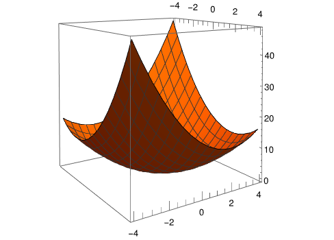
We operate a shop near the sea and sell only two products: umbrellas and bathing suits. We want to maximize our daily profit by selling the "right" combination of the two products. Suppose the temperature ranges from 50 to 95 degrees, rising from winter to summer. Sales are affected by temperature and traffic. After extensive data collection over considerable time we are able to define the profit function as you see below.
We begin with the symbolic approach. First, define
the profit function in a usual way as Revenue - Cost, and use variables x = umbrellas and y = bathing suits
To find the critical points, we take partial derivatives and equate the results to zero; solving resulting system of equations, we determine the solvion: need to sell 8 umbrellas and 11 bathing suits.
Note that a "zoom in" to plot over a smaller range reflects the familiar parabolic quadratic form which will will confirm as negative definite further below.
Now we are ready to solve numerically this optimization probl;em and plot its solution. To implement matrix operations, we approach the problem by producing a table of values the profit function might produce with different quantities of our two products.
Note the dimensions of our matrix are driven by our choice of range and range increments specified in the table.
tbl2Prod // Dimensions
{51, 51}
In order to apply the Conjugate Gradient method we build Matrix A, which is denoted as matA.
Note its Maximum is the same as our Analytical solutions optimal profit
matA = Transpose[tbl2Prod];
Max[matA]
85
The optimum is found in Row 12, Column 9 of the matrix
See matrix A in Mathematica notebook at ??????????????????????
Here is the code to execute the conjugate gradient algorithm in Wolfram language:
conjugateGradient[A_, b_, x0_, tol_ : $MachineEpsilon] := Module[
{x, residual, searchDirection, oldResidNorm, AsearchDirection,
stepSize, newResidNorm, norm},
(* Initialize the solution vector *)
x = x0;
(* Initialize residual vector *)
residual = b - A . x;
(* Initialize search direction vector *)
searchDirection = residual;
(* Norm function to compute the Euclidean norm *)
norm[v_] := Sqrt[v . v];
(* Compute initial squared residual norm *)
oldResidNorm = norm[residual];
(* Iterate until convergence *)
While[oldResidNorm > tol,
AsearchDirection = A . searchDirection;
stepSize =
oldResidNorm^2/(searchDirection . AsearchDirection);
(* Update solution *)
x = x + stepSize searchDirection;
(* Update residual *)
residual = residual - stepSize AsearchDirection;
newResidNorm = norm[residual];
(* Update search direction vector *)
searchDirection =
residual + (newResidNorm/oldResidNorm)^2 searchDirection;
(* Update squared residual norm for next iteration *)
oldResidNorm = newResidNorm;
];
x
]
■
End of Example 5
A self-adjoint matrix
is positive definite if and only if all its eigenvalues are positive.
Then the
condition number (which is ∥A−1∥ ∥A∥ for any consistent matrix norm) of A is given by \( \displaystyle \quad \kappa = \frac{\lambda_{\max}}{\lambda_{\min}} , \quad \) where λmax and λmin are the largest
and smallest eigenvalue of A.
Unfortunately, mathematicians are not consistent: a linear operator is called positive if all its eigenvalues are positive. This definition from functional analysis does not require matrix A (as operator) to be self-adjoint (A = A✶).
Throughout this section we assume that the matrix A ∈ ℝn×n is symmetric positive definite, that is, A = A✶ and ⟨x∣A x⟩ > 0 for x ≠ 0.
When A is real
symmetric (A = A✶ = AT), we have ⟨x , A x⟩ = ⟨A x∣x⟩, which justifies the Dirac notation: ⟨x∣A∣x⟩ for ⟨x∣A x⟩.
For any real symmetric positive definite square matrix A (A = A✶ = AT), we can define an A-inner product
that satisfies regular inner product laws. Two vectors x and y are called A-orthogonal or A-conjugate if
\[
\langle \mathbf{x} \mid \mathbf{y} \rangle_A = \langle \mathbf{x} \mid {\bf A}\,\mathbf{y} \rangle = 0 ,
\]
which we denote by x ⊥Ay.
To each A-inner product corresponds the A-norm that is usually referred to as an energy norm
When A = I, the identity matrix, we get the usual Euclidean inner product and norm in ℝn or any isomorphic to it space such as space of column vectors ℝn×1 or ℝ1×n row vectors---it does not matter which of these three spaces are in use.
Let A be a symmetric real square matrix. A set of vectors S = {v₁, v₂, … , vn} is called A-orthogonal or A-conjugate with respect to matrix A if all A-inner products
\[
\left\langle {\bf v}_i \mid \mathbf{A}\,{\bf v}_j \right\rangle = 0 \qquad \forall i \ne j .
\]
This definition does not require matrix A to be positive definite; however, in our further applications it will be necessarily. If A is zero matrix (A = 0), then any set of vectors is conjugate. If A is identity matrix (A = I), then conjugacy is equivalent to the usual notion of orthogonality.
Lemma 1:
Let A be symmetric and positive definite real square matrix. If set of vectors S = {v₁, v₂, … , vn} is A-conjugate, then this set is linearly independent.
We prove by contradiction If one vector from set S is a linear combination of other vectors
\[
\mathbf{v}_n = \alpha_1 \mathbf{v}_1 + \alpha_2 \mathbf{v}_2 + \cdots + \alpha_{n-1} \mathbf{v}_{n-1}
\]
with at least one nonzero coefficient, say α₁, then
\[
0 < \left\langle \mathbf{v}_n \mid \mathbf{A}\,\mathbf{v}_n \right\rangle = \alpha_1 \left\langle \mathbf{v}_n \mid \mathbf{A}\,\mathbf{v}_1 \right\rangle + \alpha_2 \left\langle \mathbf{v}_n \mid \mathbf{A}\,\mathbf{v}_2 \right\rangle + \cdots + \alpha_{n-1} \left\langle \mathbf{v}_n \mid \mathbf{A}\,\mathbf{v}_{n-1} \right\rangle = 0.
\]
Example 6:
Positive definite matrix that s not symmetric + complex
The conjugate gradient method is the algorithm that chooses search directions by A-orthogonalizing the residual against all previous search directions.
Actually, it is based on two fundamental ideas. The starting point is to replace the linear algebra problem of solving system of linear equations A x = b by equivalent optimization problem; so solution x✶ of linear system is a unique minimum of a special quadratic function.
Although there exist infinite many functions having a minimizer x✶ that satisfies the linear equation A x✶ = b. it is convenient to consider a quadratic function mainly because its gradient is equal to A x − b.
Theorem 1:
The vector x is a solution to the positive definite linear system
A x = b if and only if x
produces the minimal value of the quadratic function
The minimum value of function ϕ is \( \displaystyle \quad \phi \left( {\bf A}^{-1} {\bf b} \right) = -\frac{1}{2}\,\langle {\bf b} \mid {\bf A}^{-1} {\bf b} . \rangle . \)
Let x and v ≠ 0 be fixed column vectors of size n and let λ be a real number. We have
\begin{align*}
\phi \left( \mathbf{x} + \lambda\, \mathbf{v} \right) &= \frac{1}{2}\,\left\langle \mathbf{x} + \lambda\, \mathbf{v} \mid {\bf A} \left( \mathbf{x} + \lambda\, \mathbf{v} \right) \right\rangle - \left\langle \mathbf{x} + \lambda\, \mathbf{v} \mid {\bf b} \right\rangle
\\
&= \frac{1}{2}\,\left\langle \mathbf{x} \mid {\bf A} \,\mathbf{x} \right\rangle + \frac{\lambda}{2}\,\left\langle \mathbf{v} \mid {\bf A} \,\mathbf{x} \right\rangle + \frac{\lambda}{2}\,\left\langle \mathbf{x} \mid {\bf A} \,\mathbf{v} \right\rangle + \frac{\lambda^2}{2}\,\left\langle \mathbf{v} \mid {\bf A} \,\mathbf{v} \right\rangle
\\
& \quad - \left\langle \mathbf{x} \mid \mathbf{b} \right\rangle - \left\langle \mathbf{v} \mid \mathbf{b} \right\rangle
\\
&= \frac{1}{2}\,\left\langle \mathbf{x} \mid {\bf A} \,\mathbf{x} \right\rangle - \left\langle \mathbf{x} \mid \mathbf{b} \right\rangle
\\
& \quad + \lambda \left\langle \mathbf{v} \mid {\bf A} \,\mathbf{x} \right\rangle - \lambda \left\langle \mathbf{v} \mid \mathbf{b} \right\rangle + \frac{\lambda^2}{2}\,\left\langle \mathbf{v} \mid {\bf A} \,\mathbf{v} \right\rangle .
\end{align*}
Hence,
\[
\phi \left( \mathbf{x} + \lambda\, \mathbf{v} \right) = \phi \left( \mathbf{x} \right) - \lambda \left\langle \mathbf{v} \mid \mathbf{b} - {\bf A}\,\mathbf{x} \right\rangle + \frac{\lambda^2}{2}\,\left\langle \mathbf{v} \mid {\bf A} \,\mathbf{v} \right\rangle .
\tag{E1.1}
\]
With x and v fixed we can define the quadratic function φ in λ by
\[
\varphi (\lambda ) = \phi \left( \mathbf{x} + \lambda\, \mathbf{v} \right) .
\]
Then φ attains a minimal value when its derivative is zero because its
λ² coefficient, ⟨v, A v⟩ is
positive. Since
\[
\varphi' (\lambda ) = \left\langle \mathbf{v} \mid \mathbf{b} - {\bf A}\,\mathbf{x} \right\rangle + \lambda \left\langle \mathbf{v} \mid {\bf A} \,\mathbf{v} \right\rangle ,
\]
the minimum occurs when λ = λ* with
\[
\lambda^{\ast} = \frac{\left\langle \mathbf{v} \mid \mathbf{b} - {\bf A}\,\mathbf{x} \right\rangle }{\left\langle \mathbf{v} \mid {\bf A} \,\mathbf{v} \right\rangle} = \frac{\left\langle \mathbf{v} \mid \mathbf{b} \right\rangle - \left\langle \mathbf{v} \mid \mathbf{x} \right\rangle_A}{\| \mathbf{v} \|^2_{A}}.
\]
From Eq.(E1.1), we get
\begin{align*}
\varphi \left( \lambda^{\ast} \right) &= \phi \left( \mathbf{x} + \lambda^{\ast} \mathbf{v} \right)
\\
&= \phi \left( \mathbf{x} \right) - \lambda^{\ast} \left\langle \mathbf{v} \mid \mathbf{b} - {\bf A}\,\mathbf{x} \right\rangle + \frac{\lambda^{\ast}}{2} \left\langle \mathbf{v} \mid {\bf A} \,\mathbf{v} \right\rangle
\\
&= \phi \left( \mathbf{x} \right) - \frac{\left\langle \mathbf{v} \mid \mathbf{b} - {\bf A}\,\mathbf{x} \right\rangle }{\left\langle \mathbf{v} \mid {\bf A} \,\mathbf{v} \right\rangle} \left\langle \mathbf{v} \mid \mathbf{b} - {\bf A}\,\mathbf{x} \right\rangle + \left( \frac{\left\langle \mathbf{v} \mid \mathbf{b} - {\bf A}\,\mathbf{x} \right\rangle }{\left\langle \mathbf{v} \mid {\bf A} \,\mathbf{v} \right\rangle} \right)^2 \left\langle \mathbf{v} \mid {\bf A} \,\mathbf{v} \right\rangle /2
\\
&= \phi \left( \mathbf{x} \right) - \frac{\left\langle \mathbf{v} \mid \mathbf{b} - {\bf A}\,\mathbf{x} \right\rangle^2 }{2\,\| \mathbf{v} \|^2_{A}} .
\end{align*}
So for any vector v ≠ 0, we have
ϕ(x + λ*v) < ϕ(x) unless ⟨v∣b −A x⟩ = 0, in which case ϕ(x + λ*v) = ϕ(x).
Suppose x* satisfies A x* = b. Then ⟨v ∣ b − A x*⟩ = 0 for any vector v, and ϕ(x) cannot be made any smaller than ϕ(x*). Thus, x* minimizes ϕ.
On the other hand, suppose that x* is a vector that minimizes ϕ. Then for any vector v,
we have ϕ(x* + λ*v) ≥ ϕ(x*). Thus, ⟨v ∣ b − A x*⟩ = 0. This implies that b − A x* = 0 and consequently, that A x* = b.
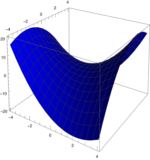
Example 7:
We consider the following function
\[
f\left( x_1 , x_2 \right) = \left( x_1 -1 \right)^2 + \left( x_2 -1 \right)^2 + \left( x_1 -1 \right)^2 \left( x_1 -2 \right)^2 + \left( x_2 -1 \right)^2 \left( x_2 -3 \right)^2 .
\]
It has the global minimum at x₁ = 1, x₂ = 1, but its gradient
\[
\nabla\,f\left( \right) = 2 \left( x_1 -1 + (x_1 -2)^2 (x_1 -1) + (x_1 -1)^2 (x_1 -2) , x_2 -1 + (x_2 -3)^2 (x_2 -1) + (x_2 -1)^2 (x_2 - 3) \right)
\]
has nothing in common with any linear system.
resembles the energy of a mechanical system; for instance, the kinetic energy of n particles with masses mi is expressed as the quadratic function of particle's coordinates:
\( \displaystyle \quad \frac{1}{2}\,\sum_{i=1}^n m_i x_i^2 . \quad \) This function ϕ
maybe considered as its generalization similar to Lyapunov's function in the theory of dynamic systems.
The minimizerx✶ of the function ϕ is given as the point where the gradient of the function is equal to zero. Direct calculations give
So the solution of the matrix/vector equation A x = b corresponds to the lowest energy state, or
equilibrium, of the system described by function ϕ.
Also, this linear algebra problem is equivalent of minimizing the A-norm of the error e = x* − x:
The last term in the identity above is independent of x, so ϕ is minimized exactly when the error is minimized. Since A is positive definite, this term \( \displaystyle \quad
\frac{1}{2} \left\| {\bf x} - {\bf x}^{\ast} \right\|_A^2 = \frac{1}{2} \left\langle \left( \mathbf{x} - \mathbf{x}^{\ast} \right) \mid {\bf A} \left( \mathbf{x} - \mathbf{x}^{\ast} \right) \right\rangle \quad \) is positive unless x − x* = 0.
The formula \eqref{EqCG.3} for ϕ shows that the same x✶ that minimizes ϕ(x) also serves as the solution to the linear system of equations A x = b. The uniques of our solution is guaranteed by the the matrix that is symmetric and positive definite.
Once we reduced the linear algebra problem A x = b to equivalent unconstrained minimization of function ϕ, we turn our attention to more sophisticated approach how to determine the minimizer x✶ of function ϕ. In order to achieve this objective, we start with an assumption that a list or array (so their order matters) of n of nonzero mutually A-conjugate vectors is known, S = [d(0), d(1), … , d(n-1)].
We postpone discussion when this list may contain less elements than the dimension of the problem to next section. If vectors in list S satisfy the A-orthogonality condition
then set S is said to be A-orthogonal.
We also abbreviate their mutual A-orthogonality as
\[
\mathbf{d}^{(0)} \perp_A \mathbf{d}^{(1)} \perp_A \cdots \perp_A \mathbf{d}^{(n-1)}
\]
Using orthogonality of list S, we can expand the true solution x✶ of the system of equations A x = b as
To determine the coefficients αk (k = 0, 1, … , n−1) of this expansion, we multiply both sides of Eq.\eqref{EqCG.5} by A d(k) for some particular index k and take inner product. This yields
that does not contain unknown vector x✶. Disadvantage of evaluation of x✶ according to Eq.\eqref{EqCG.5} becomes clear: it requires utilization of a lot of memory, especially when n is large. In practice, vectors in array S are not known in advance and should be determined according to some procedure,
for instance, conjugate Gram--Schmidt algorithm. This leads to an ill-posed problem of implementing full-history procedure by keeping in memory all previous steps (the old search vectors).
A remedy to avoid numerical instability of maintaining conjugancy of vectors in list S is to transfer summation problem into an iteration problem. One step iteration scheme was proposed in 1952 by Hestenes & Steifel:
where x(0) is an arbitrary vector, the scalar αi is the step size, and d(k) are referred to as the search direction or descent direction vector. For residuals r(k) = b − A x(k), we have a similar recurrence
At each iterative step, the only one previous information is used to define the next iterative value according to formula \eqref{EqCG.6}. Therefore, at the end of recursive procedure, we get the required solution x(n) = x✶ (subject that all calculations are performed in exact arithmetics, no roundoff).
As it is seen from one-step nonstationary inhomogeneous recurrence \eqref{EqCG.6}, the conjugate gradient algorithm generates a sequences of vectors,
{x(k)}, that always converges (when all calculations are done with exact arithmetic) to the true solution x* of the linear system A x = b. Your question is anticipated: why recurrence \eqref{EqCG.6} always converges? The answer follows from observation that list S form a basis in n dimensional vector space ℝn×1 ∋ x✶.
However, recurrence \eqref{EqCG.6} contains two unknown ingradients: parameter αi and vector d(i), which is called the search direction or descent direction vector. Therefore, the conjugate gradient method involves essentially two phases: choosing a descent
direction and picking up a point along that direction (which is identified by parameter αi).
Theorem 2:
Let A ∈ ℝn×n be positive definite, let
S = [d(0), d(1), … , d(n-1)] be an A-orthogonal list of nonzero vectors. Then step size in formula \eqref{EqCG.6} is
\[
\alpha_i = \frac{\left\langle \mathbf{d}^{(i)} \mid {\bf b} - {\bf A}\, \mathbf{x}^{(i)} \right\rangle}{\left\langle \mathbf{d}^{(i)} \mid {\bf A}\, \mathbf{d}^{(i)} \right\rangle} = \frac{\left\langle \mathbf{d}^{(i)} \mid \mathbf{r}^{(i)} \right\rangle}{\left\| \mathbf{d}^{(i)} \right\|_A^2} , \qquad i = 1,2,\ldots , n .
\]
Step size αi must be chosen in such a way to ensure that
the energy norm of error ∥ei∥A is minimized
along the descent direction, which is equivalent to determine a minimizer of function ϕ. If we fix vectors x = x(k) and d = d(k), this is equivalent minomization of function
φ(α) = ϕ(x + αd) along one dimensional line. Taking derivative, we obtain
\[
\frac{\text d}{{\text d}\alpha}\,\varphi (\alpha ) = \nabla \phi (\mathbf{x} + \alpha\mathbf{d}) \bullet \frac{\text d}{{\text d}\alpha} \left( \mathbf{x} + \alpha\mathbf{d} \right) = \nabla \phi (\mathbf{x} + \alpha\mathbf{d}) \bullet \mathbf{d} .
\]
We know from previous observations that
\[
\nabla \phi (\mathbf{x} ) = - \mathbf{r} = {\bf A}\, \mathbf{x} - \mathbf{b} .
\]
.
Hence,
\[
\nabla \phi (\mathbf{x} + \alpha \mathbf{d}) = {\bf A}\left( \mathbf{x} + \alpha \mathbf{d} \right) - \mathbf{b} = - \mathbf{r} + \alpha {\bf A} \,\mathbf{d} ,
\]
where r = b &mimus; A x is the residual vector. Therefore,
\[
\varphi' \left( \alpha \right) = - \left\langle \mathbf{r}^{(i)} \mid \mathbf{d}^{(i)} \right\rangle + \alpha \left\langle \mathbf{d}^{(i)} \mid {\bf A}\,\mathbf{d}^{(i)} \right\rangle = 0 .
\]
This leads to required formula.
The main challenge in determination of search vectors d(i) is how to maintain conjugancy of vectors in list S automatically without keeping in memory all previous step information (which is needed to avoid ill-posed problem).
Theorem 3:
Let A ∈ ℝn×n be positive definite, let x ∈ ℝn×1, and let S be a subspace of ℝn×1. Then there is a unique s ∈ ℝn×1 such that
\[
\| \mathbf{x} - \mathbf{s} \|_A = \min_{\mathbf{u} \in S} \| \mathbf{x} - \mathbf{u} \|_A .
\]
The vector s is A-orthogonal to S, so s ⊥Au for every u ∈ S.
Let β = [v₁, v₂, … , vn] be an A-orthogonal basis of the vector space ℝn×1 such that first k vectors of it [v₁, v₂, … , vk] constitute a basis of vector subspace S ⊆ ℝn×1. So subspace S and its complement S⊥ are spanned on disjoint subsets:
\[
S = \mbox{span} \left[\mathbf{v}_1 , \mathbf{v}_2 , \ldots , \mathbf{v}_k \right] , \quad S^{\perp} = \mbox{span}\left[\mathbf{v}_{k+1} , \mathbf{v}_{k+2} , \ldots , \mathbf{v}_n \right] .
\]
Such A-orthogonal basis exists because any basis (linear independent list of vectors) can be transformed into A-conjugate basis using conjugate Gram--Schidt process.
Let x ∈ ℝn×1 be an arbitrary column vector. Then it can be expressed in unique way as a linear combination of elements from basis β:
\[
\mathbf{x} = c_1 \mathbf{v}_1 + c_2 \mathbf{v}_2 + \cdots + c_k \mathbf{v}_k + c_{k+1} \mathbf{v}_{k+1} + \cdots + c_n \mathbf{v}_n .
\]
Let
\[
\mathbf{s} = c_1 \mathbf{v}_1 + c_2 \mathbf{v}_2 + \cdots + c_k \mathbf{v}_k \in S
\]
and
\[
\mathbf{s}^{\perp} = c_{k+1} \mathbf{v}_{k+1} + c_{k+2} \mathbf{v}_{k+2} + \cdots + c_n \mathbf{v}_n \in S^{\perp} .
\]
Therefore, any vector x can be uqiquely written as x = s + s⊥ so that s ∈ S and s⊥ ∈ S⊥.
To see that this decomposition is unqie, let us assume the opposite: x = r + r⊥with r ∈ S and r⊥ ∈ S⊥. Then the equation x = s + s⊥ = r + r⊥ implies that z = s − r = r⊥ − s⊥. Thus, z ∈ S ∩ S⊥ = {0} and we conclude that z = 0, which means s = r and s⊥ =
r⊥.
The unique elements s and s⊥ are called the A-orthogonal projections of x into S and S⊥, respectively. When vectors s and s⊥ are A-orthogonal, then the conjugate Pythagorian theorem holds:
\[
\left\| \mathbf{s} + \mathbf{s}^{\perp} \right\|^2_A = \| \mathbf{s} \|_A^2 + \left\| \mathbf{s}^{\perp} \right\|^2_A .
\]
Indeed
\[
\[
\left\| \mathbf{s} + \mathbf{s}^{\perp} \right\|^2_A = \left\langle \mathbf{s} + \mathbf{s}^{\perp} \mid \mathbf{s} + \mathbf{s}^{\perp} \right\rangle_A = \left\langle \mathbf{s} \mid \mathbf{s} \right\rangle_A + \left\langle \mathbf{s}^{\perp} \mid \mathbf{s}^{\perp} \right\rangle_A ,
\]
because ⟨s ∣ s⊥⟩A = ⟨s⊥ ∣ s⟩A = 0.
Now suppose that there exists another w ∈ S such that x − w ∈ S⊥. Then decomposition x = w + (x − w) would violate the uniquenes of decomposition of x into two parts, one from S and another from its complement, S⊥. Then vector s satisfies conditions of this theorem. Indeed, since x − s = (x − u) + (u − s), where x − u ∈ S⊥ and u − s ∈ S, we have
\[
\left\| \mathbf{x} - \mathbf{s} \right\|_A^2 = \left\| \mathbf{x} - \mathbf{u} \right\|_A^2 + \left\| \mathbf{u} - \mathbf{s} \right\|_A^2 .
\]
As s runs through S, the term ¶lell;x − u∥² remains constant, while the term ¶lell;u − s∥² variues but remains strictly positive wzxwpt that it equals zero when u = s. Thus, ¶lell;x − s∥² is minimized when and only when s = u.
Example 8:
■
End of Example 8
A naïve approach is to choose the n coordinate directions in ℝn as search directions, that is, d(k) =
ek, where ek is the kth standard orthonormal basis vector for k = 1, 2, … , n. Then this approach (in n steps) provides a one step in the Gauss–Seidel method.
An iterative method to choose the residuals r(k) = b − A x(k) = −∇ϕ(x(k)) as the search directions is called the method of steepest descent. However, the resulting iterative method may exhibit a poor performance for many functions
ϕ whose graph is a long, narrow valley. In particular, the local minimization point x(k+1) may situate at a point where that line is tangent to the level sets of ϕ.
Consequently, the
next search direction r(k+1), being orthogonal to the level sets at x(k+1) , must be
orthogonal to the old search direction r(k). This geometry often causes the iterative
method to take many short, inefficient switchbacks down to the valley floor, when a
better choice of search directions could lead to a more direct descent.
The relationship between the linear system A x = b and the minimization of function ϕ(x) inspires a geometric interpretation as well as a physical one.
From multivariable calculus, it follows that the residual vector r points in the direction of the steepest descent of ϕ, as
illustrated for the case n = 2 in the following figure.
If we denote by Si the vector space spanned on first i+1 search vectors, {d(0), d(1), … , d(i)}, then we see that every next iterate vector x(i) must be A-orthogonal to the i-dimensional affine space
\( \displaystyle \quad \mathbf{x}^{(0)} + S_{i-1} \ \) because d(i) is conjugate to it.
tells us that its minimization is the same as minimization of the energy norm of the error. So at every step, we need to solve one-dimensional minimization problem along the line spanned on the search vector d(i) according to Eq.\eqref{EqCG.6}. What makes the conjugate gradient method outstanding is that it remembers information from past steps so that it minimizes a higher dimensional problem by minmizing one dimensional problem over vector space spanned on properly chosen the descent vector.
To identify the search directions, we need a definition.
A vector x(k) is said to be optimal with respect to a
direction d ≠ 0 if
\[
\phi \left( {\bf x}^{(k)} \right) \leqslant \phi \left( {\bf x}^{(k)} + \lambda\,{\bf d}\right) , \qquad \forall \lambda \in \mathbb{R} .
\]
If x(k) is optimal with respect to any direction in a vector space V, we say that x(k) is optimal with respect to V.
From the definition of optimality, it turns out that d must be orthogonal
to the residual r(k). Indeed, from the definition, we conclude that ϕ(x(k) + λd) admits a local
minimum along d for λ = 0, and thus the partial derivative of ϕ with
respect to λ must vanish at λ = 0. Since
for some vector q. Let us assume that x(k) is optimal with respect to a direction d (thus, r(k) ⊥ d). Let us impose that x(k+1) is still optimal with respect to d, that is, r(k+1) ⊥ d. We obtain
A method employing A-conjugate descent directions is called conjugate.
The next step is how to generate automatically a sequence of conjugate
directions. The conjugate gradient method of Hestenes and Stiefel chooses the search directions { d(k) } during the iterative process so that the residual vectors { r(k) } are mutually orthogonal. To achieve this, it is appropriate to apply the conjugate Gram--Schmidt process to the next residual vector by subtracting the orthogonal projection on the line generated by the descent vector:
Solving the latter with respect to βk, we obtain formula \eqref{EqCG.8}. Note that the residual vector r(k+1) is A-orthogonal to all previous descent directions except d(k).
The recurrence relation \eqref{EqCG.7} makes conjugate gradient method so formidable because it secures A-orthogonality of all search directions, but not only two sequential ones.
The conjugate gradient method generates two sequences of vectors, x(k) and d(k), k = 0, 1, 2, …. The first sequence always converges (when all calculations are done with exact arithmetic) to the true solution x* = A−1b of the system A x = b. The second sequence is used to determine the iterates at every step
Here the vector d(i) is the search direction and the scalar αi is the step size.
At each iterative step, the only one of these directions is used to define the next iterative value according to the formula \eqref{EqCG.6}.
ϕ 𝔎
The conjugate gradient method generates a finite set of A-orthogonal search directionsd(0), d(1), … , d(n-1) by picking up a point of local minimum for ϕ along that direction:
The search directions are A-orthogonal and nonzero as long as the residuals are linearly independent (equivalently, nonzero).
Now it is right time to appreciate the beauty of CG-algorithm proposed by Hestenes & Steifel. It efficiently bypasses full-history recurrence of the Gram--Schmidt process and convert it into the one-step iterative algorithm:
Conjugate Gradient Algorithm:x(0) is given
r(0) = b − A x(0)d(0) = r(0)
do until converged for k = 1, 2, 3, …
αk = ⟨r(k) ∣ d(k)⟩/⟨d(k) ∣ Ad(k)⟩ step length
x(k+1) = x(k) + αkd(k) approximate solution
r(k+1) = r(k) − αkA d(k) residual
if ∥r(k)∥ is less than some tolerance, then stop
βk = ⟨r(k+1) ∣ A d(k)⟩/⟨d(k) ∣ A d(k)⟩ improvement of this step
d(k+1) = r(k+1) − βkd(k) search direction
Example 9:
We consider a linear system A x = b with
\[
{\bf A} = \begin{bmatrix} 15&9&8&-6&-4 \\
9&19&-3&-7&-3 \\
8&-3&19&8&-10 \\
-6&-7&8&16&-4 \\
-4&-3&-10&4&15
\end{bmatrix} , \qquad {\bf b} = \begin{pmatrix} 13 \\ -5 \\ 41 \\ 48 \\ 19 \end{pmatrix} ,
\tag{9.1}
\]
has the exact solution x✶ (x✶₁, x✶₂, x✶₃, x✶₄, x✶₅) = (1, 2, 3, 4, 5), which we check with Mathematica:
Since we want to apply conjugate gradient method, we need to check first whether matrix A is symmetric and positive definite. Using Mathematica, we find
So Mathematica gives us a green light for CG utilization.
To apply the conjugate gradient method, we pick up an initial guess x(0) = (0, 0, 0, 0, 0). Since b = (13, −5, 41, 48, 19), the initial residual is r(0) = b - A x(0) = b.
Since size of matrix A is small, we can find its inverse, and they apply to b.
Inverse[A]
The solving the given equation exactly, we get
Inverse[A].b
To perform the first iteration, we need to calculate two parameters (α₁, β₁) and search vector d(1):
\[
\alpha_0 = \frac{\left\langle \mathbf{r}^{(0)} \,\mid\, \mathbf{d}^{(0)} \right\rangle}{\left\langle \mathbf{d}^{(0)} \,\mid\, {\bf A}\,\mathbf{d}^{(0)} \right\rangle} = \frac{2270}{44447} \approx 0.0510721 ,
\]
Example 10:
We consider a linear system
\[
\begin{cases}
2\,x+3\,y -z &= 11 .
\\
3\,x + y -2\,z &= 9 .
\\
x -3\,y + 4\,z &= 1,
\end{cases}
\tag{10.1}
\]
that has a nonsymmetric matrix
\[
{\bf A} = \begin{bmatrix} 2&\phantom{-}3&-1 \\ 3&\phantom{-}1&-2 \\ 1&-3&\phantom{-}4 \end{bmatrix} \in \mathbb{R}^{3\times 3} , \qquad {\bf b} = \begin{bmatrix} 11 \\ 9 \\ 1 \end{bmatrix} \in \mathbb{R}^{3\times 1} .
\]
Then we can rewrite system (10.1) in concise form A x = b.
This system has
the exact solution x✶ (x✶, y✶, z✶) = (3, 2, 1). Since matrix A for system (9.1) is not symmetrical, we multiply both sides of equation
A x = b by transposed matrix AT. This yields a new system B x = f.with a new symmetric matrix
\[
{\bf B} = {\bf A}^{\mathrm T} {\bf A} = \begin{bmatrix} 14&\phantom{-}6&-4 \\ \phantom{-}6& \phantom{-}19& -17 \\ -4& -17& \phantom{-}21 \end{bmatrix} , \qquad {\bf f} = {\bf A}^{\mathrm T} {\bf b} = \begin{bmatrix} \phantom{-}50 \\ \phantom{-}39 \\-25 \end{bmatrix} \in \mathbb{R}^{3 \times 1} .
\tag{10.2}
\]
A = {{2, 3, -1}, {3, 1, -2}, {1, -3, 4}}
B = Transpose[A] . A
f = Transpose[A] . {11, 9, 1}
{50, 39, -25}
Since matrix B is symmetric, we need to check whether this matrix is positive definite. So using Mathematica, we find its eigenvalues
N[Eigenvalues[B]]
{39.0093, 12.2868, 2.70396}
Since eigenvalues of matrix B are positive, we can apply the conjugate gradient method to solve system B x = f.
\[
\lambda_1 \approx 39.009 , \quad \lambda_2 \approx 12.2868 , \quad \lambda_3 \approx 2.70396 .
\]
To apply the conjugate gradient method, we pick up an initial guess x(0) = (0, 0, 0). Since f = (50, 39, −25), the initial residual vector is r(0) = f - B x(0) = f = (50, 39, -25). The initial search vector is equal to the residual: d(0) = f.
B = {{14, 6, -4}, {6, 19, -17}, {-4, -17, 21}};
f = {50, 39, -25}
x0 = {0, 0, 0};
r0 = f
d0 = f
{50, 39, -25}
To perform the first iteration, we need to calculate two parameters (α₁, β₁) and search vector d(1):
\[
\alpha_0 = \frac{\left\langle \mathbf{r}^{(0)} \mid \mathbf{r}^{(0)} \right\rangle}{\left\langle \mathbf{d}^{(0)} \mid {\bf B}\,\mathbf{d}^{(0)} \right\rangle} = \frac{2323}{71787} , \qquad \mathbf{r}^{(1)} = \mathbf{r}^{(0)} - \alpha_0 {\bf B}\, \mathbf{d}^{(0)} = \frac{1}{71787} \begin{bmatrix} 1187368 \\ 605825 \\ 1429649 \end{bmatrix} .
\]
All properties of the conjugate gradient algorithm are formulated for exact arithmetic because errors associated with machine arithmetic can destroy the conjugancy and orthogonality relationships. . Hence, the final residual vector r(n) may never vanish in actual calculations. Moreover, in many settings, the size of the problem n is a large number, so we would like to stop iterating after much smaller number of iterations, which motivates the derivation of error estimates for the conjugate gradient method.
Lemma 2:
Let A ∈ ℝn×n be symmetric and positive definite. Let x(k+1) = x(k) + αkd(k) be obtained from an exact line search. Then residuals are A-orthogonal to the previous search vectors, that is,
\begin{align}
&\left\langle \mathbf{r}^{(i)} \,\mid \,{\bf A}\, \mathbf{d}^{(j)} \right\rangle
=\left\langle \mathbf{r}^{(i)} \,\mid \,\mathbf{d}^{(j)} \right\rangle_A
\notag
\\
&= \begin{cases}
\frac{1}{\alpha_i}\,\left\langle \mathbf{r}^{(i)} \,\mid \,\mathbf{r}^{(i)} \right\rangle , & \quad \mbox{if} \quad i = j ,
\\
\frac{-1}{\alpha_{i-1}}\,\left\langle \mathbf{r}^{(i)} \,\mid \,
\mathbf{r}^{(i)} \right\rangle , & \quad \mbox{if} \quad i = j+1 ,
\\
0 , & \quad \mbox{otherwise}.
\end{cases}
\label{EqCG.10}
\end{align}
We use induction on the size of indices i, j. When i, j ≤ 1, proposition holds by construction of the initial algorithm's step. Assume that the proposition is valid whenever i, j ≤ k for some integer k ≥ 1. We show that the statement is true for i, j ≤ k+1 by establishing the following claim. For j = 0, 1, 2, … , k, ⟨rk+1 ∣ d(j) ⟩ = 0.
Using the recurrence for residuals, r(k+1) = r(k) − αkA d(k), we obtain
\[
\left\langle \mathbf{r}^{(k+1)} \,\mid\, \mathbf{d}^{(k)} \right\rangle = \left\langle \mathbf{r}^{(k)} - \alpha_k {\bf A}\,{\bf d}^{(k)} \,\mid\, \mathbf{d}^{(k)} \right\rangle = 0
\]
because step size αk is chosen according to formula (9) to satisfy this equation.
Example 11:
We consider a linear system A x = b, where
\[
\mathbf{A} = \begin{bmatrix} 873& -2162& 462 \\ -2162& 5361& -1146 \\ 462& -1146& 245 \end{bmatrix} , \qquad \mathbf{b} = \begin{pmatrix} -2065 \\ 5122 \\ -1095 \end{pmatrix} .
\]
We check with Mathematica that matrix A is positive definite.
Since the residual vector is zero, we stop CG iteration.
■
End of Example 11
Corollary 1:
Let A ∈ ℝn×n be symmetric and positive definite. Let x(k+1) = x(k) + αkd(k) be obtained from an exact line search. Then the error vectors e(k) = x✶ − x(k) = A−1b − x(k)
satisfy the recurrence
\[
\mathbf{e}^{(k+1)} = \mathbf{e}^{(k)} - \alpha_k \mathbf{d}^{(k)} , \qquad k =0, 1, 2 , \ldots ;
\]
because A e(k+1) = r(k+1), k = 0, 1, ….
The error at each step is conjugate to all of the previous search directions:
\[
\mathbf{e}^{(j)} \perp_A \mathbf{d}^{(i)} = 0 , \qquad
\mbox{for} \quad i = 0, 1, \ldots , j-1 .
\]
We use induction on the size of indices i, j. When i, j ≤ 1, proposition holds by construction of the initial algorithm's step. Assume that the proposition is valid whenever i, j ≤ k for some integer k ≥ 1. We show that the statement is true for i, j ≤ k+1 by establishing the following claim. For j = 0, 1, 2, … , k, ⟨rk+1 ∣ d(j) ⟩ = 0.
Using the recurrence for residuals, r(k+1) = r(k) − αkA dsup>(k), we obtain
\[
\left\langle \mathbf{r}^{(k+1)} \,\mid\, \mathbf{d}^{(k)} \right\rangle = \left\langle \mathbf{r}^{(k)} - \alpha_k {\bf A}\,{\bf d}^{(k)} \,\mid\, \mathbf{d}^{(k)} \right\rangle = 0
\]
because step size αk is chosen according to formula (9) to satisfy this equation.
Example 12:
■
End of Example 12
Lemma 3:
If A ∈ ℝn×n is symmetric and positive definite, then distincs search vectors are A-conjugate:
\[
\mathbf{d}^{(i)} \perp_A \mathbf{d}^{(j)} =0 \quad \iff \quad \left\langle \mathbf{d}^{(i)} \,\mid\, {\bf A}\,\mathbf{d}^{(j)} \right\rangle = 0 \quad\mbox{for} \quad i\ne j .
\]
We use induction on the size of indices i, j. When i, j ≤ 1, proposition holds by construction of the initial algorithm's step. Assume that the proposition is valid whenever i, j ≤ k for some integer k ≥ 1. We show that the statement is true for i, j ≤ k+1 by establishing the following claim. For j = 0, 1, 2, … , k, ⟨rk+1 ∣ d(j) = 0.
Using the Gram--Schmidt process applied to the energy inner product, we obtain
\[
\mathbf{d}^{(k+1)} = \mathbf{r}^{(k+1)} - \sum_{i=0}^k \left( \frac{\left\langle \mathbf{r}^{(k+1)} \,\mid\, \mathbf{d}^{(i)} \right\rangle_A}{\left\langle \mathbf{d}^{(i)} \,\mid\, \mathbf{d}^{(i)} \right\rangle_A} \right) \mathbf{d}^{(i)} .
\]
Example 13:
■
End of Example 13
Lemma 4:
If A ∈ ℝn×n is symmetric and positive definite, then distincs residuals are orthogonal:
\[
\mathbf{r}^{(i)} \perp \mathbf{r}^{(j)} =0 \quad \iff \quad \left\langle \mathbf{r}^{(i)} \,\mid\, \mathbf{r}^{(j)} \right\rangle = 0 \quad\mbox{for} \quad i\ne j .
\]
Example 14:
■
End of Example 14
Theorem 4:
Step size coefficients αk and βk can be evaluated alternatavely as long as d(i) ≠ 0,
where r(k) = b − Ax(k) is the residual vector. Also,
\[
\beta_i = - \frac{\left\langle {\bf r}^{(i+1)} \mid {\bf r}^{(i+1)} \right\rangle}{\left\langle {\bf r}^{(i)} \,\mid\,{\bf r}^{(i)} \right\rangle} = - \frac{\left\| {\bf r}^{(i+1)} \right\|^2}{\left\| {\bf r}^{(i)} \right\|^2}, \qquad i =0,1,2,\ldots , n-1 .
\tag{8a}\]
From recurrence (7), it follows that
\[
\left\langle \mathbf{d}^{(k+1)} \mid \mathbf{r}^{(k+1)} \right\rangle = \left\langle \mathbf{r}^{(k+1)} \mid \mathbf{r}^{(k+1)} \right\rangle = \left\| \mathbf{r}^{(k+1)} \right\|^2_2
\]
because all previous descent vectors d(i) are orthogonal to the residual vector r(k+1) for i = 0, 1, … , k.
Example 15:
■
End of Example 15
The conjugate gradient method has a memory in the sense that, at every step, it maintains conjugancy of all previously obtained search vectors and not the single one preceding entry. In order to maintain this orthogonality, we need to subtract from the residual r(k+1) all previously obtained search vectors that constructed by the Gram--Schmidt process:
where every term \( \quad \left( \frac{\left\langle \mathbf{r}^{(k+1)} \,\mid\, \mathbf{d}^{(i)} \right\rangle_A}{\left\langle \mathbf{d}^{(i)} \,\mid\, \mathbf{d}^{(i)} \right\rangle_A} \right) \mathbf{d}^{(i)} \quad \) is the projection of the residual vector r(k+1) on the descent direction vector d(i).
Fortunately, all coefficients in this sum are zeroes except the last one because
Thus, ⟨ r(k) ∣ d(k) ⟩ > 0 as long as r(k) ≠ 0. This implies that d(k) ≠ 0.
Theorem 5:
Let A ∈ ℝn×n be symmetric and positive definite. After m steps of the conjugate gradient algorithm (with r(k) ≠ 0 at each previous step), we have
\begin{align*}
\mbox{span}\left\{ \mathbf{d}^{(0)} , \mathbf{d}^{(1)} , \ldots , \mathbf{d}^{(m)} \right\} &= \mbox{span}\left\{ \mathbf{r}^{(0)} , \mathbf{r}^{(1)} , \ldots , \mathbf{r}^{(m)} \right\}
\\
&= \mbox{span}\left\{ \mathbf{r}^{(0)} , {\bf A}\,\mathbf{r}^{(0)} , \ldots , {\bf A}^m \mathbf{r}^{(0)} \right\} .
\end{align*}
Proof by induction on m. When m = 0, the proposition is trivial because d(0) = r(0). Assume that the assessment is valid up to m = k. By residual update equation r(m) = r(m-1) − αm-1<A d(m-1), we have
\[ \mathbf{r}^{(k+1)} = \mathbf{r}^{(k)} - \alpha_k {\bf A}\,\mathbf{d}^{(k)} \] and the inductive hypothesis ensures that d(k) ∈ span{r(0), … , Akr(0)}.
Example 16:
■
End of Example 16
Theorem 6:
Let x(k+1) = x(k) + αkd(k) be obtained by an exact line search that minimizes ϕ:
\[
\phi \left( {\bf x}^{(k+1)} \right) = \min_{\alpha \in \mathbb{R}} \,\phi \left( {\bf x}^{(k)} + \alpha\,{\bf d}^{(k)} \right) .
\]
where step size is evaluated according to Eq.(9).
Let φ(α) = ϕ(x(k) + α d(k)).
We can find out αk as being the value
of the parameter α such that ϕ(x(k) + α d(k)) is minimized. Differentiating
with respect to α and setting to zero the derivative at the minimizer, yields
Example 17:
■
End of Example 17
Corollary 2:
If the method maintains conjugancy for all search direction vectors, then the error e(m) satisfy the following inequality:
\[
\left\| \mathbf{e}^{(m)} \right\|_A = \min_{\mathbf{d} \in S_m} \left\|
\mathbf{e}^{(0)} - \mathbf{d} \right\|_A ,
\]
where Sm = span{d(0), d(1), … , d(m-1)}.
Theorem 7:
Let [d(0), d(1), … , d(n-1)]
be an A-orthogonal list of nonzero vectors associated with the positive
definite matrix A, and let x(0) be arbitrary. Define
step size αk according ro formula (9) for k = 1, 2, … , n. Then, assuming exact arithmetic, A x(n) = b.
Since, for each k = 0, 1, 2, … , n−1, x(k+1) = x(k) + αkd(k), we have
\begin{align*}
{\bf A}\,\mathbf{x}^{(n)} &= {\bf A}\,\mathbf{x}^{(n-1)} + \alpha_{n-1}{\bf A}\,\mathbf{x}^{(n-1)}
\\
&= \left( {\bf A}\,\mathbf{x}^{(n-2)} + \alpha_{n-2}{\bf A}\,\mathbf{x}^{(n-2)} \right) + \alpha_{n-1}{\bf A}\,\mathbf{x}^{(n-1)}
\\
\vdots & \qquad \vdots \qquad\qquad \qquad \vdots \\
\\
&= {\bf A}\,\mathbf{x}^{(0)} + \alpha_0 {\bf A}\,\mathbf{d}^{(0)} + \alpha_1 {\bf A}\,\mathbf{d}^{(1)} + \cdots + \alpha_{n-1} {\bf A}\,\mathbf{d}^{(n-1)}
\end{align*}
Subtracting b from this result yields
\[
{\bf A}\, \mathbf{x}^{(n)} - \mathbf{b} = {\bf A}\, \mathbf{x}^{(0)} - \mathbf{b} + \alpha_0 {\bf A}\, \mathbf{d}^{(0)} + \alpha_1 {\bf A}\, \mathbf{d}^{(1)} + \cdots + \alpha_{n-1} {\bf A}\,\mathbf{d}^{(n-1)}
\]
We now take the inner product of both sides with the vector d(k) and use the properties of inner products and the fact that A is symmetric to obtain
\begin{align*}
\left\langle {\bf A}\,\mathbf{x}^{(n)} - \mathbf{b} \mid \mathbf{d}^{(k)} \right\rangle &= \left\langle {\bf A}\,\mathbf{x}^{(0)} - \mathbf{b} \mid \mathbf{d}^{(k)} \right\rangle + \alpha_0 \left\langle {\bf A}\,\mathbf{d}^{(0)} \mid \mathbf{d}^{(k)} \right\rangle + \cdots
\\
& \quad + \alpha_{n-1} \left\langle {\bf A}\,\mathbf{d}^{(n-1)} \mid \mathbf{d}^{(k)} \right\rangle
\\
&= \left\langle {\bf A}\,\mathbf{x}^{(0)} - \mathbf{b} \mid \mathbf{d}^{(k)} \right\rangle + \alpha_{k} \left\langle {\bf A}\,\mathbf{d}^{(k)} \mid \mathbf{d}^{(k)} \right\rangle
\end{align*}
because direction vectors are mutually A-conjugate. However, αk ⟨ d(k) ∣ A d(k) ⟩ =
αk ⟨ d(k) ∣ b − A d(k-1) ⟩. Hence,
\begin{align*}
\alpha_k \left\langle \mathbf{d}^{(k)} \,\mid\,{\bf A}\, \mathbf{d}^{(k)} \right\rangle &= \left\langle \mathbf{d}^{(k)} \,\mid\,\mathbf{b} - {\bf A}\, \mathbf{d}^{(0)} + {\bf A}\, \mathbf{d}^{(0)} - {\bf A}\, \mathbf{d}^{(1)} + \cdots \right.
\\
& \quad \left. - {\bf A}\, \mathbf{d}^{(k-2)} + {\bf A}\, \mathbf{d}^{(k-2)} - {\bf A}\, \mathbf{d}^{(k-1)} \right\rangle
\\
&= \left\langle \mathbf{d}^{(k)} \,\mid\,{\bf b} - {\bf A}\, \mathbf{d}^{(0)} \right\rangle + \left\langle \mathbf{d}^{(k)} \,\mid\, {\bf A}\, \mathbf{d}^{(0)} - {\bf A}\, \mathbf{d}^{(1)} \right\rangle + \cdots
\\
& \quad + \left\langle \mathbf{d}^{(k)} \,\mid\, {\bf A}\, \mathbf{d}^{(k-2)} - {\bf A}\, \mathbf{d}^{(k-1)} \right\rangle .
\end{align*}
We knpw that for any i
\[
\mathbf{x}^{(i)} = \mathbf{x}^{(i-1)} + \alpha_{i-1} \mathbf{d}^{(i-1)} \qquad \Longrightarrow \qquad {\bf A}\,\mathbf{x}^{(i)} = {\bf A}\,\mathbf{x}^{(i-1)} + {\bf A}\, \alpha_{i-1} \mathbf{d}^{(i-1)} ,
\]
so
\[
{\bf A}\, \mathbf{x}^{(i-1)} - {\bf A}\, \mathbf{x}^{(i)} = - \alpha_{i-1}{\bf A}\, \mathbf{d}^{(i-1)}
\]
Thus,
\[
\left\langle \mathbf{d}^{(k)} \,\mid\, {\bf A}\, \mathbf{d}^{(k)} \right\rangle = \left\langle \mathbf{d}^{(k)} \,\mid\, {\bf b} - {\bf A}\, \mathbf{x}^{(0)} \right\rangle - \alpha_1 \left\langle \mathbf{d}^{(k)} \,\mid\, {\bf A}\, \mathbf{d}^{(1)} \right\rangle - \cdots - \alpha_{k-1} \left\langle \mathbf{d}^{(k)} \,\mid\, {\bf A}\, \mathbf{d}^{(k-1)} \right\rangle
\]
Because of the A-orthogonality, ⟨ d(k) ∣ A d(j) ⟩ = 0 for k ≠ j, so
\[
\left\langle \mathbf{d}^{(k)} \,\mid\, {\bf A}\, \mathbf{d}^{(k)} \right\rangle = \left\langle \mathbf{d}^{(k)} \,\mid\, {\bf b} - {\bf A}\, \mathbf{x}^{(0)} \right\rangle
\]
Using equation
\[
\left\langle {\bf A}\,\mathbf{x}^{(n)} - {\bf b} \,\mid \,\mathbf{d}^{(k)} \right\rangle = \left\langle {\bf A}\,\mathbf{x}^{(0)} - {\bf b} \,\mid \,\mathbf{d}^{(k)} \right\rangle + \alpha_k \left\langle {\bf A}\,\mathbf{d}^{(k)} \,\mid \,\mathbf{d}^{(k)} \right\rangle
\]
we obtain
\begin{align*}
\left\langle \mathbf{d}^{(k)} \,\mid\,{\bf A}\, \mathbf{x}^{(n)} - {\bf b} \right\rangle &= \left\langle \mathbf{d}^{(k)} \,\mid\,{\bf A}\, \mathbf{x}^{(0)} - {\bf b} \right\rangle
+ \left\langle \mathbf{d}^{(k)} \,\mid\,{\bf b} - {\bf A}\, \mathbf{x}^{(0)} \right\rangle
\\
&= \left\langle \mathbf{d}^{(k)} \,\mid\,{\bf A}\, \mathbf{x}^{(0)} - {\bf b} \right\rangle - \left\langle \mathbf{d}^{(k)} \,\mid\,{\bf A}\, \mathbf{x}^{(0)} - {\bf b} \right\rangle
\\
&= 0 .
\end{align*}
Hence the vector A x(n) − b is orthogonal to the A-orthogonal list of vectors [d(0), d(1), … , d(n-1)]. Therefore, A x(n) − b = 0.
Example 18:
The linear system
\[
\begin{cases}
4\,x+3\,y \phantom{+4\,x} &= 13 .
\\
3\,x + 4\,y -z &= 16 .
\\
\phantom{4\,x} -y + 2\,z &= -5,
\end{cases}
\tag{18.1}
\]
has the exact solution x✶ (x✶, y✶, z✶) = (1, 3, −1).
To apply the conjugate gradient method, we pick up an initial guess x(0) = (0, 1, 1). Since b = (13, 16, −5), the initial residual is r(0) = b - A x(0) = (10, 13, -6)
because
\[
{\bf A} = \begin{bmatrix} 4&3&0 \\ 3&4&-1 \\ 0&-1&2 \end{bmatrix} , \quad {\bf b} = \begin{bmatrix} 13 \\ 16 \\ -5 \end{bmatrix} , \quad {\bf r}^{(0)} = {\bf d}^{(0)} = \begin{bmatrix} 10 \\ 13 \\ -6 \end{bmatrix} .
\]
A = {{4, 3, 0}, {3, 4, -1}, {0, -1, 2}};
b = {13, 16, -5};
x0 = {0, 1, 1};
r0 = b - A . x0
{10, 13, -6}
To perform the first iteration, we need to calculate two parameters (α₁, β₁) and search vector d(1):
\[
\alpha_0 = \frac{305}{2084} , \qquad \mathbf{r}^{(1)} = \mathbf{r}^{(0)} - \alpha_0 {\bf A}\, \mathbf{d}^{(0)} = \frac{1}{2084} \begin{bmatrix} 3255 \\ 252 \\ 4879 \end{bmatrix} .
\]
There is no need to perform further calculations.
■
End of Example 18
Theorem 8:
Let A be an n-by-n symmetric and positive definite matrix. In exact arithmetic, the conjugate gradient method for solving system A x = b
converges after at most n steps. Moreover, the error ek = x✶ − x(k) at the
kth iteration (with k < n) is orthogonal to search vector d(j) for j = 0, 1, 2, … , k − 1 and
\[
\left\| \mathbf{e}_k \right\|_A \leqslant \frac{2\,c^k}{1 + c^{3k}} \, \left\| \mathbf{e}_0 \right\|_A ,
\]
with \( \displaystyle \quad c = \frac{\sqrt{\kappa (\mathbf{A})} -1}{\sqrt{\kappa (\mathbf{A})} +1} . \quad \) Here
\( \displaystyle \quad \kappa (\mathbf{A}) = \| \mathbf{A}^{-1} \| \,\| \mathbf{A} \| \quad \) is the condition number, which depends on choice of norm of the matrix.
LeVeque, page 78 / in pdf it is page 83
see for instance [QSS07, Chapter 4] or [Saa03].
Quarteroni A., Sacco R., and Saleri F. (2007) Numerical Math-
ematics. 2nd edition. Texts in Applied Mathematics. Springer-
Verlag, Berlin.
Saad Y. (2003) Iterative Methods for Sparse Linear Systems.
2nd edition. SIAM publications, Philadelphia, PA.
[Sal08]
Salsa S. (2008) Partial Differential Equations in Action From
Modelling to Theory. Springer, Milan.
Example 19:
■
End of Example 19
Example 20:
We build a 6 × 6 symmetric positive definite matrix with the aid of Kronecker product. First, we choose some orthogonal matrices of dimensions 3 and 2:
\[
{\bf B}_3 = \frac{1}{3} \begin{bmatrix} 2&-2&1 \\ 1&2&2 \\ -2&-1&2 \end{bmatrix} , \qquad {\bf C}_2 = \frac{1}{5} \begin{bmatrix} 3&4 \\ 4&-3 \end{bmatrix} .
\]
Now we consider the linear system A x = b, where
\[
\mathbf{b} = \begin{bmatrix} 89& 552& 643& 924& 1261& 1248 \end{bmatrix}^{\mathrm T} .
\tag{20.2}
\]
This system has a unique solution
\[
\mathbf{x}^{\ast} = \begin{bmatrix} 1& 2& 3& 4& 5& 6 \end{bmatrix}^{\mathrm T} .
\tag{20.3}
\]
as Mathematica confirmed:
LinearSolve[A, b]
{1, 2, 3, 4, 5, 6}
Now we are ready to apply the conjugate gradient method for solving system of linear equations A x = b with matrix (20.1) and input data (20.2). WE start with an initial guess x(0) = 0 and make some preliminary calculations:
When a square n=by-n matrix A is ill-conditioned, the
conjugate gradient method is highly susceptible to rounding errors. So, although the exact
answer should be obtained in n steps, this is not usually the case. As a direct method the
conjugate gradient method is not as good as Gaussian elimination with pivoting. The main
use of the conjugate gradient method is as an iterative method applied to a better-conditioned
system. In this case an acceptable approximate solution is often obtained in about √n steps.
Darve, E. and Wootters, M., Numerical Linear Algebra with Julia, SIAM, Philadelphia, 2021.
Watkins, D.S., Fundamentals of Matrix Computations, Wiley; 3rd edition, 2010.
White, R.E., Computational Linear Algebra with Applications and MATLAB Computations, CRC Press Boca Raton, FL, 2023. doi: 10.1201/9781003304128
Barrett, R., Berry, M., Chan, T., Demmel, J., Donato, J., Dongarra, J.,
Eijkhout, V., Pozo, R., Romine, C., and van der Vorst, H., Templates for the Solution of Linear
Systems: Building Blocks for Iterative Methods, SIAM, Philadelphia, Pennsylvania, 1993.
Darve, E. and Wootters, M., Numerical Linear Algebra with Julia, SIAM, Philadelphia, 2021.
Krylov, A. N. (1931). "О численном решении уравнения, которым в технических вопросах определяются частоты малых колебаний материальных систем" [On the Numerical Solution of Equation by Which are Determined in Technical Problems the Frequencies of Small Vibrations of Material Systems]. Izvestiia Akademii Nauk SSSR (in Russian). 7 (4): 491–539.
Hestenes, Magnus R.; Stiefel, Eduard (December 1952). "Methods of Conjugate Gradients for Solving Linear Systems" (PDF). Journal of Research of the National Bureau of Standards. 49 (6): 409. doi:10.6028/jres.049.044
Lanczos, C. (1950). "An iteration method for the solution of the eigenvalue problem of linear differential and integral operators" (PDF). Journal of Research of the National Bureau of Standards. 45 (4): 255–282. doi:10.6028/jres.045.026
Loehr, N., Advanced Linear Algebra, CRC Press, 2014.
Shi, X., Wei, Y., and Zhang, W., Convergence of General Nonstationary Iterative Methods for Solving Singular Linear Equations, Taylor & Francis Online, Volume 38, Issue 11,