Throughout ℂ stands for the set of all complex numbers. If z = x + ⅉy ∈ ℂ, its complex conjugate is denoted by z✶ = x − ⅉy, where ⅉ or j denotes the imaginary unit, so ⅉ² = −1.
Holomorphic functions
We consider functions of complex variable z ∈ ℂ defined on some domain Ω ⊂ ℂ. We also expect that f(z) will in general take values in &Co
pf; as well.
If f(z) = u + ⅉv, then the function u(x, y) is called the real part of f and
v(x, y) is called the imaginary part of f. Of course, it will not in general be possible to plot the graph of f(z), which will lie in ℂ², the set of ordered
pairs of complex numbers, that is the set {(z,w) ∈ ℂ²
: w = f(z)}. The graph can also be viewed as the subset of ℝ4
given by {(x, y, s, t): s = u(x, y), t = v(x, y)}. In particular, it lies in a four-dimensional space.
If z = x + ⅉy,
then a function f(z) is simply a function f(x, y) = u(x, y)+ ⅉv(x, y) of the two real variables x and y. As such, it is a function (mapping) from ℝ² to ℝ².
The usual operations on complex numbers extend to complex functions:
given a complex function f(z) = u + ⅉv, we can define functions Re f(z = u (the real part is also denoted by ℜ), Im f(z = v (the imaginary part is also denoted by ℑ), complex conjugate f✶(z = u − ⅉv, \( \displaystyle \quad |f(z)| = \sqrt{u^2 + v^2} . \quad \) Likewise, if g(z) is another complex-valued function, we can define f(z) g(z) and f(z)/g(z) provided g(z) ≠ 0.
Example 1:
A polynomial is an expression of the form
ⅉ
where the 𝑎i are complex numbers, and it defines a function in the usual way. It can be shown that the real and imaginary parts of a polynomial P(z) are polynomials in x and y. For example,
2 I x + (2 - 4 I) x^2 + (3 + 2 I) x^4 -
2 y + (8 + 4 I) x y - (8 - 12 I) x^3 y - (2 - 4 I) y^2 - (18 +
12 I) x^2 y^2 + (8 - 12 I) x y^3 + (3 + 2 I) y^4
However, given two (real) polynomial functions u(x, y) and v(x, y), it is very rarely the
case that there exists a complex polynomial P(z) such that P(z) = u + ⅉv.
For example, it can be seen that x cannot be of the form P(z), nor can z✶. As we shall see later, no polynomial in x and y taking only real values for
every z (i.e. v = 0) can be of the form P(z). Of course, since x = ½(z + z✶) and y = ½(z + z✶)/ⅉ in z and
z✶, i.e.,
The absolute value measures the distance between two complex numbers.
Thus, z₁ and z₂ are close when |z₁ − z₂| is small. We can then define the
limit of a complex-valued function f(z) as follows: we write
\[
\lim_{z\to c} \ f(z) = C ,
\]
where c and C are understood to be complex numbers, if the distance from f(z) to C, |f(z) − C|, is small whenever |z − c| is small. More precisely,
if we want |f(z) − C| to be less than some small specified positive real number ε, then there should exist a positive real number δ such that, if |z − c| < δ, then |f(z) − C| < ε. Note that, as with real functions, it does
not matter if f(c) = C or even that f(z) be defined at c. It is easy to see
that, if c =(c₁, c₂), C = 𝑎 + ⅉb and f(z) = u + ⅉv is written as real and imaginary parts, then \( \displaystyle \quad \lim_{z \to c} \ f(z) = C \quad \)
if and only if \( \displaystyle \quad \lim_{(x,y) \to (c_1 ,c_2 )}\ u(x,y) = a \quad\mbox{and} \quad \lim_{(x,y) \to (c_1 ,c_2 )}\ v(x,y) = b . \quad \) Thus, the story for limits of functions of a complex
variable is the same as the story for limits of real valued functions of the
variables x, y. However, a real variable x can approach a real number c only from above or below (or from the left or right, depending on your point of
view), whereas there are many ways for a complex variable to approach a
complex number c.
Sequences, limits of sequences, convergent series and power series can be
defined similarly.
As for functions of a real variable, a function f(z) is continuous at c if
\[
\lim_{z\to c} \ f(z) = f(c) .
\]
In other words, the limit exists, f(·) is defined at z = c, and its value at c is the limiting value. A function f(·) is continuous in some domain Ω ⊆ ℂ if it is continuous at all points z ∈ Ω. It means that a function f(z) = u + ⅉv
is continuous if and only if its real and imaginary parts are continuous; so
that the usual functions z, z✶, Rez, Imz, |z|, ez are continuous.
z
are continuous
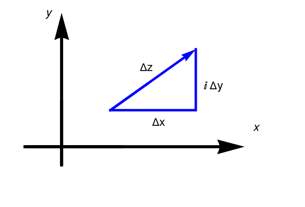
if it exists. Here z = 𝑥 + ⅉy is a complex number and ⅉ or j is the imaginary unit in the complex plane ℂ, so ⅉ² = −1. In Δz = Δ𝑥 + ⅉΔy, Δ𝑥 and Δy are independent of each other.
Thus, approaching 0 along horizontal and vertical directions has given two
different expressions. Equating real and imaginary parts, we see that: if a function f(z) = u + ⅉv is complex differentiable, then its real and imaginary parts satisfy the Cauchy-Riemann equations:
Likewise, f(z) = x² + ⅉy² does not. Note that the Cauchy-Riemann equations
are two equations for the partial derivatives of u and v, and both must be
satisfied if the function f(z) is to have a complex derivative.
■
End of Example 2
We have seen that a function with a complex derivative satisfies the
Cauchy--Riemann equations. In fact, the converse is true:
Theorem 1:
Let f(z) = u + ⅉv be a complex-valued function defined in a region Ω (open subset) of ℂ, and suppose that u and v have continuous first partial derivatives with respect to x and y. If u and v satisfy the Cauchy-Riemann
equations, then f(z) has a complex derivative.
Take an arbitrary point z₀ = x₀ + ⅉy₀ ∈ Ω. We want to prove that
\[
f' (z_0 ) = \lim_{\Delta z\to 0} \ \frac{f(z_0 +\Delata z ) - f(z_0 )}{h}
\]
exists.
Write 7Deltaz = z − z₀ = h + ⅉk, where h = x − x₀ and k = y − y₀. Then
Thus the complex derivative exists at z₀. Since z₀ was arbitrary,
\[
\fbox{$f \mbox{ is complex differentiable throughout }\Omega$} .
\]
Why the continuity assumption matters?
The Cauchy–Riemann equations alone are not sufficient in general to guarantee complex differentiability. The continuous first partial derivatives ensure that u and v are differentiable as functions of two real variables, which lets us control the error term o(|z − z₀|).
An equivalent formula for the derivative is
The crucial step is that the Cauchy–Riemann equations make the real-variable linear approximation of f equal to multiplication by the single complex number ux+ⅉvx. That is exactly what is needed for a complex derivative.
Theorem 2:
Let f(z) = u + ⅉv be a holomorphic function.
If f′(z) is identically zero, then f(z) is a constant.
If either Ref(z) = u or Imf(z) = v is constant, then f(z) is constant.
In particular, a nonconstant holomorphic function cannot take only real or
only pure imaginary values.
If |f(z)| is constant or argf(z) is constant, then f(z) is constant.
''
Example 1:
■
End of Example 1
Write the function f(z) in the form u + ⅉv:
\[
(a)\ 5z + \mathbf{j}z , \qquad (b)\ z^{\ast}/z , \qquad (c) \ 1/z .
\]
If f(z) = ez, describe the images under f(z) of horizontal and vertical
lines, i.e. what are the sets f(𝑎 + ⅉt) and f(t + ⅉb), where 𝑎 and b are real constants and t runs through all real numbers?
Is the function z✶/z continuous at 0? Why or why not? Is the function z✶/z
holomorphic where it is defined? Why or why not?
Compute the derivatives of the following holomorphic functions, and be
prepared to justify your answers:
\[
(a)\ \frac{\left( 2 - 3\mathbf{j} \right) z - 4\mathbf{j}}{z^2 + \left( 1- \mathbf{j}\right) z + 3 - 2\mathbf{j}} , \qquad (b)\ \frac{1}{e^z - e^{-z}} , \qquad (c)\ e^{z^2} .
\]
Let f(z) = u + ⅉv be holomorphic. Recall that the Jacobian is the function
given by the following determinant:
\[
\frac{\partial (u,v)}{\partial (x,y)} = \begin{vmatrix}
\partial u/\partial x &\partial u/\partial y \\ \partial v/\partial x &\partial v/\partial y \end{vmatrix} .
\]
Using the Cauchy-Riemann equations, show that this is the same as |f(z)|².
Let f(z) be a complex-valued function. Is it possible for both f(z) and its complex conjugate f✶(z) to be holomorphic?
Apostol, T.M., Calculus, Vol. 2: Multi-Variable Calculus and Linear Algebra with Applications to Differential Equations and Probability, Wiley; 2nd edition, 1991; ISBN-13: 978-0471000075.