Example: Consider a population of field mice who inhabit a certain rural area. Suppose that several owls live in the same neighborhood and they kill 15 mice per day. Then the mouse population P(t), t is measured in months, satisfies the differential equation
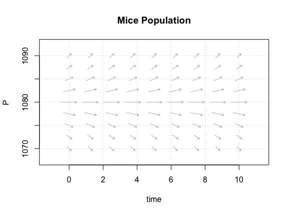
Solution: In order to solve this problem and first find equilibrium solutions where slope is zero. Upon equating islope to zero, \( P/3 - 360 =0, \) we find that P = 1080 is the critical point, also called the stationary solution. To plot our solution around P = 1080 on Rstudio, we need to import R’s phaseR package. Please note that to solve your equation, you do still need the deSolve package. Next, we write the code, as below:
library(phaseR)

apma1 <- function(t, y, parameters){
    a <- parameters[1]
    dy <- a*((y/3) - 360)
    list(dy)
}

apma1.flowField <- flowField(apma1, xlim = c(0, 10),
                             ylim    = c(1070, 1090), parameters = c(1),
                             points = 9, system = "one.dim",
                             add = FALSE, xlab = "time", ylab = "P",
                             main = "Mice Population")

grid()
There are few new elements in the code above, namely the flowField command, which plots one or two dimensional autonomous ODE systems and is in phaseR, thus our system in our code is one dimensional. Next, we see new assignments for the limits on x and y. In this code, I put our t, or time, ranging from 0 to 10, while our y, or P, is either 10 units above or below 1080, our equilibrium solution. The add command sets our equation to FALSE because if TRUE our plot is added to an existing plot, while FALSE logically implies the creation of a new plot. Moreover, I set the label for the x-axis as time as while I set the y-axis as P. I set the points to 9 because that is the number of directions fields drawn in the plotting. You can experiment and see the graph that appeals to you the most, but I chose a reasonable but random 9 in this case. Lastly, grid() adds rectangular grids to our plot. Below is our coding in Rstudio and the subsequent direction field plot.

We plot the slope field for the differential equation
