Return to computing page for the first course APMA0330
Return to computing page for the second course APMA0340
Return to computing page for the fourth course APMA0360
Return to Mathematica tutorial for the first course APMA0330
Return to Mathematica tutorial for the second course APMA0340
Return to Mathematica tutorial for the fourth course APMA0360
Return to the main page for the course APMA0330
Return to the main page for the course APMA0340
Return to the main page for the course APMA0360
Introduction to Linear Algebra with Mathematica
is Fredholm in appropriate Sobolev paces. Krupchyk--Tuomela (Cambridge University Press) states that elliptic BVPs are well-posed only if the boundary conditions satisfy the SL condition.
For a fixed point on the boundary, x⁰ ∈ ∂Ω, we cmhoose local coordinates so that xₙ is the outward normal and the boundary is xₙ = 0. Freeze coefficients at x⁰ and take the tangential Fourier transform in x′ = (x₁, x₂, … , xn−1):
This is the "microscopic boundary test" where the SL conditin checks for non-trivial decaying solutions of the transformed ODE. Ellipticity of A ensures that the characteristic polynomial in the normal direction has exactly m/2 roots with positive imaginary part, giving a space of decaying solutions of dimension m/2.
The boundary conditions Bj satisfy the Shapiro--LOpatinskii condition at x⁰ if for every ξ′ ≠ 0,
the only decaying solution v(xₙ) of the model ODE satisfying \( \displaystyle \quad B_{j, m_j} (\mathbf{x}^0 , \xi' , \texttt{D}_n )\,v(0) = 0 \quad\) for all j is the trivial solution.
Equivalently, the boundary symbol map B(x⁰, ξ′) is injection (one-to-one).
If the SL condition holds at every boundary point, then
the boundary value problem is Fredholm (finite-dimensional kernel and cokernel),
solutions satisfy full elliptic regularity,
the BVP is well-posed in Sobolev spaces.
The Lopatinskii (or Shapiro–Lopatinskii) determinant is an algebraic tool used to check if a boundary value problem (BVP) for an elliptic partial differential equation is well-posed (meaning it forms a Fredholm operator yielding regular solutions). It tests whether the boundary conditions are "compatible" with the interior differential operator. The core idea of its construction is as follows.
Freeze and Fourier Transform: Fix a point on the boundary. Map the local boundary to a flat hyperplane where y = xₙ > 0
is the interior and xₙ = 0
is the boundary. Apply a partial Fourier transform to the tangential directions (ξ′ ∈ ℝⁿ), leaving a ordinary differential equation (ODE) in the normal direction (xₙ).
Find Decay Solutions: For a fixed tangential frequency ξ′ ≠ 0, find all stable solutions to the principal symbol ODE that decay as xₙ → ∞. For a second-order equation like the Laplacian, this space of stable solutions is 1-dimensional.
Apply Boundary Symbols: Plug this stable solution into the principal symbols of your boundary conditions.
The Determinant: The Lopatinskii determinant is the determinant of the resulting linear system.
If the determinant is non-zero for all ξ′ ≠ 0, the boundary condition covers the operator perfectly. The problem is elliptic, yielding finite-dimensional kernels/cokernels and smooth solutions.
If the system is overdetermined (more boundary conditions than stable solution dimensions), the boundary matrix is non-square (more rows than columns). A non-square matrix cannot yield a unique solution for arbitrary vectors, meaning it lacks a well-defined, non-vanishing determinant, and the condition structurally fails.
Example 1:
Consider Ω = {xₙ > 0} ⊂ ℝⁿ, and the Laplace operator
Decaying solution as y = xₙ → +∞ is
\( \displaystyle \quad v(x_n ) = C\, e^{- |\xi' | x_n} = C\, e^{- |\xi' | y} , \quad \) so dim(N+) = 1 = m/2.
Dirichlet boundary condition:
\[
B\,u = u\big\vert_{x_n =0} .
\]
For any non-zero tangential frequency ξ′ ≠ 0, the general solution that decays as xₙ → ∞ is \( \displaystyle \quad v\left( x_n \right) = C\,e^{-|\xi' |\,x_n} . \quad \) This means the space N+ of stable, decaying solutions is 1-dimensional (spanned by e−|ξ′}y, where y = xₙ). The single constant C represents the degree of freedom.
Plugging our decaying solution v(y) = Ce−|ξ′|y into the boundary condition gives
Boundary symbol on the space of decaying solutions N+ is
\[
B(\xi' )\left( v \right) = v(0) = C\cdot 1.
\]
So the Lopatinskii matrix is just 1-by-1 matrix 〚 1 ⟧ with determinant 1. The standard Shapiro--Lopatinskii condition holds. The problem is strictly elliptic and well-posed (Hadamard well-posed).
This operator is injective on N+
\[
v(0) = 0 \qquad \Longrightarrow \qquad C = 0 \qquad \Longrightarrow \qquad v \equiv 0 .
\]
Evaluating derivative of function that decays at infinity, \( \displaystyle \quad v \left( x_n \right) = C\, e^{- |\xi' |\,x_n} , \)
\[
- v' (y) = |\xi' |\,C\,e^{- |\xi' |y} , \qquad y = x_n , l
\]
yields its symbol:
\[
B_N (\xi' ) = -v' (0) = |\xi' |\,C .
\]
This is again 1-by-1 matrix ⟦ξ′⟧; its (Lopatinskii) determinant is not zero for all ξ′ ≠ 0.
The SL condition holds everywhere except at the zero frequency (ξ′ = 0), which corresponds to the global kernel/constant solutions). The problem is well-posed up to a constant.
\[
\partial_{x_n} v(0) = -| \xi' |\,C .
\]
Too many boundary condiutions (failure of Cauchy problem for Δ):
We consider Laplace's equation Δu = f subject to the Cauchy initial conditions along one independent variable (say xₙ)
\[
B_D u = u \big\vert_{x_n = 0} = g_D (\mathbf{x}'), \qquad B_N u = \partial_{x_n} u \big\vert_{x_n = 0} = g_N (\mathbf{x}') .
\]
is still injective, but not bijection because the number of constraints (2) exceeds the dimension of the stable solution space (1), the Lopatinskii matrix is not square, but 1×2.
Algebraically, this makes the boundary principal symbol to be non-square matrix (specifically overdetermined). In the system framework, we check the linear independence of the boundary requirements relative to the space of stable solutions
Since the system cannot be uniquely solved for a general boundary data vector, the Lopatinskii determinant fails to be a bijection, violating the condition.
When you study the Laplacian in a domain Ω
with both Dirichlet and Neumann conditions given on the entire boundary,
This demands that\( \displaystyle \quad -|\xi' |\,\hat{g}_D - \hat{g}_N = 0 , \quad \) implying that the Dirichlet and Neumann data cannot be chosen independently for a stable solution.
You are dealing with an overdetermined problem (specifically, a Cauchy problem for an elliptic equation). It is severely ill-posed in the sense of Hadamard.
The kernel represents the "degrees of freedom" left over—the non-zero solutions to the completely homogeneous problem (f = 0 inside Ω and gD = 0, gN = 0). In our case, the kernel is trivial (ker = {0}) because by the unique continuation property of harmonic functions, if a function satisfies Δu = 0
inside a connected domain, and both its value (u = 0) and normal derivative (∂u/∂n = 0) vanish on the boundary, the function must be identically zero everywhere in the domain.
Takeaway: The operator is injective. If a solution exists, it is completely unique.
The cokernel represents the "missing space" or the infinite constraints your data (f, gD, gN) must satisfy for a solution to exist.
The cokernel has infinite dimension.
Why: For standard elliptic problems (like Dirichlet alone), the cokernel is finite-dimensional. But here, because you are over-constraining the system, arbitrary choices for gD
and gN
will almost never yield a solution. Green’s identities impose massive global constraints linking the data. For instance, if f = 0, the data must satisfy:
for every harmonic function v
in the domain. Because there are infinitely many independent harmonic functions v, there are infinitely many constraints on your boundary data.
By definition, an operator is defined as a Fredholm operator if and only if it has a finite-dimensional kernel and a finite-dimensional cokernel.
However, in the context of partial differential equations (PDEs), there is an essential topological detail that must be met to ensure this definition functions properly: the image (range) of the operator must be closed.
We create an operator A that
maps a function u
to its interior Laplacian and its simultaneous boundary values:
Let Ω ⊂ ℝⁿ be a bounded domain with smooth boundary ∂Ω. Let H¹(Ω) be the standard Sobolev space of functions on Ω. By the Trace Theorem, the boundary restriction operators map H¹(Ω)
onto specific fractional Sobolev spaces on the boundary
.
Dirichlet Trace Operator γ₀ : H¹(Ω) → H½(∂Ω), defined by γ₀(u) = u|∂Ω;
Neumann Trace Operator: γ₁ : H¹(Ω) → H−½(∂Ω), defined by \( \displaystyle \quad \left. \frac{\partial u}{\partial\mathbf{n}} \right\vert_{\partial\Omega} , \quad \) where n is unit outward normal vector.
For any given Dirichlet data g ∈ H½(∂Ω), there is a unique harmonic solution u ∈ H¹(Ω) such that γ₀u = g, where γ₀ is the projection on ∂Ω. We can define the Dirichlet-to-Neumann (Poincaré-Steklov) operator:
\[
\Lambda\, g = \gamma_1 u \quad \mbox{where } \Delta u = 0 \mbox{ in } \Omega \quad\mbox{and } \gamma_0 u = g .
\]
Λ is a classical elliptic pseudodifferential operator of order 1. It is a bounded, bijective operator (modulo constants).
In the Cauchy problem, we seek a harmonic function u ∈ H¹(ω) satisfying both γ₀u = g
and γ₁u = h. We define the Cauchy boundary operator
acting on the space of harmonic functions ℋL ⊂ H¹(ω):
To see why coker(T)
is infinite-dimensional, we look at how "small" the image Im(T)
is relative to the target space.
Let {eₖ}, k = 1, 2, …,
be the orthonormal basis of 𝔏²(∂Ω)
consisting of the eigenfunctions of the positive Laplace-Beltrami operator −Δ∂Ω
on the boundary, with eigenvalues λₖ → ∞.
The operator Λ
behaves like (−Δ∂Ω)½
at high frequencies. Specifically, for large k:
\[
\Lambda\,e_k = \sqrt{\lambda_k}\.e_k .
\]
The standard Sobolev norms on the boundary for a function ϕ = ∑ cₖeₖ are given by \( \displaystyle \quad \| \phi \|^2_{H_s} \,\sim\,\sum |c_k |^2 \left( 1 + \lambda_k \right)^s . \quad \) Let's test an arbitrary pairs of target data (g, h) ∈ H½(∂Ω) × H−½(∂Ω), decomposed into this basis
For (g, h)
to belong to Im(T), it must satisfy hₖ = Λgₖ ≈ √λₖ gₖ for every k.
Now, construct an infinite set of linearly independent vectors vj = (0, ej) in the target space H½(∂Ω) × H−½(∂Ω)
Each vj clearly belongs to H½(∂Ω) × H−½(∂Ω) because 0 ∈ H½(∂Ω) and ej ∈ H−½(∂Ω).
For any finite linear combination \( \displaystyle \quad \sum_{j=0}^m \alpha_j \mathbf{v}_j = \sum_{j=0}^m \alpha_j \left( o, e_j \right) , \quad \) the only way this vector lands in Im(T) is if ∑ αjej = Λ(0) = 0, which forces all αj = 0.
Consequently, the infinite-dimensional subspace {0} × H−½(∂Ω)
intersects Im(T)
only at the zero vector. Because we can embed the entire infinite-dimensional space H−½(∂Ω)
into the quotient coker(T)
without any overlap with Im(T), the dimension of the cokernel is strictly infinite.
Zaremba Problem:
If your domain's boundary ∂Ω
is split into two disjoint pieces (∂Ω = ΓD ∩ ΓN), then
On ΓD
(Dirichlet alone): The Shapiro–Lopatinskii condition is satisfied.
On ΓN
(Neumann alone): The Shapiro–Lopatinskii condition is satisfied.
At the interface (ΓD ∪ ΓN): The condition fails structurally because the boundary operator transitions discontinuously. This failure is why solutions to mixed boundary value problems typically exhibit a loss of regularity (e.g., the gradient of u
blows up like r−1/2) near the interface where the conditions switch.
■
End of Example 1
For any given Dirichlet data g in Sobolev spaceH½(∂Ω), there is a unique harmonic solution u ∈ H¹(Ω) such that γ₀u = g, where γ₀ is the projection on ∂Ω. We can define the Dirichlet-to-Neumann (Poincaré-Steklov) operator:
\[
\Lambda\, g = \gamma_1 u \quad \mbox{where } \Delta u = 0 \mbox{ in } \Omega \quad\mbox{and } \gamma_0 u = g .
\]
Λ is a classical elliptic pseudodifferential operator of order 1 for bounded domain Ω ⊂ ℝⁿ with smooth boundary ∂Ω. It is a bounded, bijective operator (modulo constants).
Example 2:
To build clear analytical intuition, we assume a constant, homogeneous conductivity field σ(x) = 1. Under this assumption, the DtN map reduces to mapping a given boundary potential f
to the outward normal derivative of its harmonic extension:
where ν is the outward normal vector of unit length.
Here are three classical geometries where the DtN operator can be written explicitly using integral transforms or series expansions.
Example A: The Upper Half-Plane ℝ²+
Let the domain be the upper half-plane Ω = {x, y) ∈ &Rof;² : y > 0}. The boundary is the real axis ∂Ω = {(x, 0) : x ∈ ℝ}. The outward normal unit vector pointing out of the domain is ν = [0, −1].
For a given boundary condition u(x, 0) = f(x)
decaying at infinity, the bounded harmonic extension in the interior is given by the Poisson integral formula:
This explicitly proves that the DtN map on a flat boundary acts exactly as the square root of the Laplacian operator \( \displaystyle \quad \left( \Lambda_1 = +\sqrt{-\Delta_{\partial\Omega}} \right) , \quad \)
mapping smooth profiles to higher-frequency profiles.
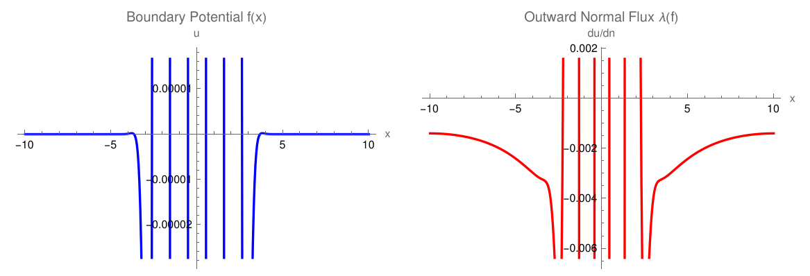
(* 1. Define Spatial Grid and Boundary Potential Function *)
dx = 0.05;
xRange = Range[-10., 10., dx];
nPoints = Length[xRange];
f[x_] := Exp[-x^2] * Cos[3 * x];
fData = Table[f[x], {x, xRange}];
(* 2. Forward FFT to Frequency Space *)
fFourier = Fourier[fData, FourierParameters -> {-1, 1}];
(* 3. Define the Multiplier Matrix |\[Xi]| for the Grid *)
frequencies = Table[
If[i <= nPoints/2, (i - 1), (i - 1 - nPoints)] * (2. * Pi / (nPoints * dx)),
{i, nPoints}
];
absFrequencies = Abs[frequencies];
(* 4. Apply the DtN Operator in Frequency Space and Inverse FFT *)
dtnFourier = absFrequencies * fFourier;
dtnData = Re[InverseFourier[dtnFourier, FourierParameters -> {-1, 1}]];
(* 5. Organize coordinates for flawless line plotting *)
plotData1 = Table[{xRange[[i]], fData[[i]]}, {i, nPoints}];
plotData2 = Table[{xRange[[i]], dtnData[[i]]}, {i, nPoints}];
(* 6. Visualize Potential vs Flux *)
plotA1 = ListLinePlot[plotData1,
PlotStyle -> Blue, PlotLabel -> "Boundary Potential f(x)", AxesLabel -> {"x", "u"}];
plotA2 = ListLinePlot[plotData2,
PlotStyle -> Red, PlotLabel -> "Outward Normal Flux \[Lambda](f)", AxesLabel -> {"x", "du/dn"}];
GraphicsRow[{plotA1, plotA2}, ImageSize -> 700]
Potential vs flux.
Example B: The Unit Disk 𝔃
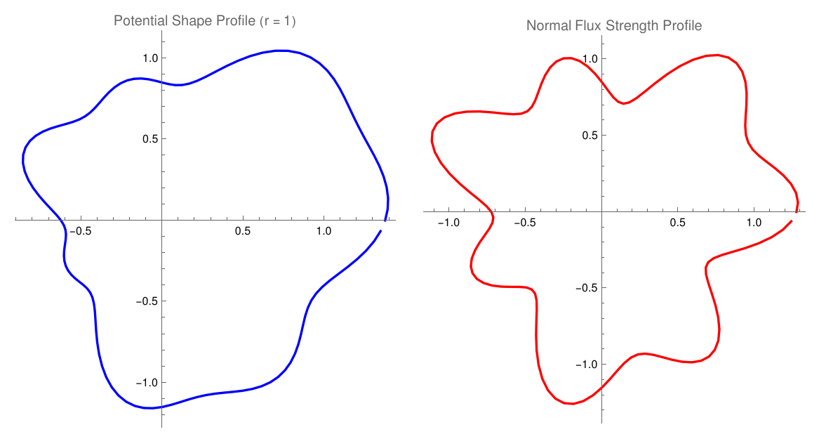
Let the domain be the unit circle Ω = {(r, θ) : r < 1}, where the boundary ∂Ω is the unit circumference r = 1. The outward normal unit vector is simply the radial direction ν = r̂.
If the boundary potential f(θ)
is represented by its Fourier series expansion:
This demonstrates that the DtN map scales each Fourier component linearly by its frequency number |n|. Higher spatial frequencies are amplified much more aggressively than lower frequencies, reinforcing why recovering microstructures deep inside a domain from boundary data is severely ill-posed.
Example C: A Wedge Domain (Infinite Sector)
Let the domain be an open wedge of opening angle α
in polar coordinates: Ω = {(r, θ) : r > 0, 0 < θ < α}. The boundary ∂Ω
consists of two semi-infinite straight rays: the bottom edge (θ = 0) and the top edge (θ = α).
The Dirichlet data f
maps to two separate distribution components: f₀(r)
along the bottom ray and fα(r)
along the top ray. By applying a Mellin Transform with respect to the radial coordinate r:
The Laplace equation transforms into an ordinary differential equation\( \displaystyle \quad \frac{{\text d}^2 \hat{u}}{{\text d} \theta^2} + s^2 \hat{u} = 0. \ \) Solving this with boundary conditions yields the explicit DtN map in the transformed Mellin frequency space:
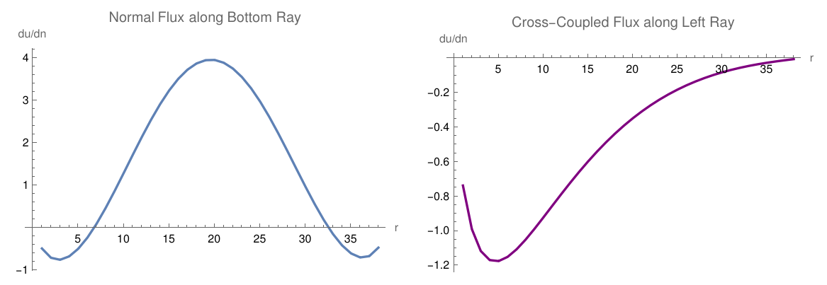
When evaluated back in physical space via an inverse transform, this manifests as a coupled system of singular integral operators mapping potentials along one edge of the wedge directly to current distributions leaking out of both edges.
For a right-angle corner domain, current leaks across both intersecting boundaries. This example uses a highly stable Finite Difference / Relaxation method to find the explicit interior harmonic extension u(x, y)
inside the wedge first, then numerically differences the boundary grid rows to plot the DtN normal derivative maps along the edges.
\[
\Gamma_1 = \left\{ x = 0, \ y> 0 \right\} , \qquad \Gamma_2 = \left\{ y = 0, \ x > 0 \right\} ,
\]
which meet at the corner (0, 0).
The classical Shapiro–Lopatinskii condition is a local smooth-boundary condition. Therefore it can
be checked on each open edge separately. The corner itself requires an additional corner analysis.
Fix a point on Γ₁.
Here x is the normal variable and y is tangential to the boundary. Take the Fourier transform only
in the tangential variable y:
Therefore the only decaying solution satisfying the homogeneous boundary condition is the trivial
solution. Hence the Shapiro–Lopatinskii condition is satisfied on Γ₁.
The same argument applies to
Γ₂ = {y = 0, x > 0}.
Now y is the normal variable and x is tangential. Fourier transforming in x gives
\[
u^F_{yy} - \xi^2 u^F = 0 .
\]
The decaying mode for y > 0 is
\[
u(\xi , y) = C\,e^{- |\xi |\,y} .
\]
The homogeneous Dirichlet condition at y = 0 gives
C = 0.
Thus, the Shapiro–Lopatinskii condition is also satisfied on Γ₂.
The same local calculation works for standard Neumann data. For example, on x = 0,
\[
u_x (+0 , y) = 0,
\]
which again forces C = 0 for nonzero tangential frequency.
The point (0, 0)
is not a smooth boundary point. Consequently, the classical Shapiro–Lopatinskii condition by itself
does not describe all possible behavior near the corner.
For a corner or wedge, one typically supplements the edgewise Shapiro–Lopatinskii analysis with a
Kondrat’ev-type corner analysis. Introduce polar coordinates
\[
x = r\,\cos\theta , \qquad y = r\,\sin\theta ,
\]
so that the quarter-plane corresponds to
\[
0 < \theta < \frac{\pi}{2} .
\]
For Laplace’s equation, seek separated corner modes of the form
These values are the characteristic corner exponents for this Dirichlet wedge problem.
For Laplace’s equation on the quarter-plane, the natural structure is
\[
\begin{array}{c}
\mbox{Shapiro–Lopatinskii condition on each smooth edge}
\\
+
\\
\mbox{Kondrat’ev/operator-pencil analysis at the corner.}
\end{array}
\]
Therefore the answer is yes: the Shapiro–Lopatinskii condition is directly applicable to Laplace’s
equation on the quarter-plane, but only along the smooth boundary portions. The corner (0, 0) is a
separate singular point and requires additional corner theory if one wants a complete regularity or
Fredholm analysis.
■
End of Example 3
Example 4:
In n-dimensional space Ω = {xₙ ≫ 0}, take the transport operator
\[
A = \paryial_y = \frac{\partial}{\partial y} , \qquad y = x_n .
\]
with general solution v(y) = C, a constant. This colution does not decay as y = xₙ → +∞. The whole SL framework (decaying subspace of dimension m/2) breks; there is no splitting into decaying/growing modes, and the "boundary symbol" cannot be defined in the usual elliptic sense.
Even if we impose a homogeneous boundary condition like v(0) = 0, the interior non-elliptic means:
the operator is not Fredholm,
solutions are not regular in the elliptic sense,
SL is simply not applicable.
This example illustrates that elliptocity of the interior operator is a prerequisite: without it, the characteristic roots do not give a finite dimensional decaying subspace, and the SL condition cannot be formulated meaningfully.
■
End of Example 4
Example 5:
Let A = Δ² be the biharmonic operator, which is of order 4. Upon application of tangential Fourier transform, we get
which is a fourth order ODE. The corresponding characteristic equation has double roots λ = ±|ξ′|, each of multiplicity 2. The set of decaying solutions is spanned on \( \displaystyle \quad \left\{ e^{-|\xi' |\,y} , \ y\,e^{-|\xi' |\,y} \right\} , \quad \) where y = xₙ. Therefore, the space of decaying solutions N+ has dimension 2 = m/2.
Now we consider a
clamped plate (Dirichlet + normal derivative):
So this particular choice still satisfies SL. To actually break SL, we need boundary operators whose principal parts are linearly dependent on 𝑁+. For example, take only one condition:
\[
B\,u = \partial_n u \big\vert_{x_n = 0}
\]
Then B(ξ′) : 𝑁+ → C has 2-dimensional domain and 1‑dimensional codomain, hence non‑injective: there exists a nontrivial v ∈ 𝑁+ with ∂ₙv(0) = 0. Therefore, there are too few independent boundary conditions ⇒ SL fails.
■
End of Example 5
Example 6:
In n-dimensional space (n is either 2 or 3), displacement
𝑢 : Ω → ℝⁿ, the Lamé operator (or Lamé-Navier operator) is
On the half‑space { 𝑥ₙ > 0 }, after tangential Fourier transform, one obtains a matrix ODE system in 𝑥ₙn
\[
A_2 (\xi' , \partial_n )\,v(x_n ) = 0 ,
\]
whose characteristic roots split into one longitudinal and
𝑛−1 transverse modes, each with decaying exponent \( \displaystyle \quad e^{-|\xi' |y} , \quad \) where y = xₙ.
Altogether, dim𝑁+ = n = 𝑚/2 for the system.
Traction (natural) boundary conditions:
Let 𝜎(𝑢) ,be the stress tensor, and impose the boundary operator
On the decaying modes, the boundary symbol is an
𝑛×𝑛 matrix depending on 𝜉′, and for strongly elliptic Lamé parameters; it is invertible for all 𝜉′≠0. This is the classical result: Lamé with traction boundary conditions satisfies SL.
Mixed or incomplete boundary conditions (failure of SL)
If we impose, say, only one scalar condition on the vector field u (e.g. only the normal component of displacement vanishes, but tangential components are unconstrained), then the boundary symbol map
\[
B(\xi' ) \ : \ N^{+} \mapsto C
\]
cannot be injective (domain dimension 𝑛 > 1), so there exist nontrivial decaying solutions satisfying the boundary condition.
Incomplete boundary conditions for Lamé ⇒ SL fails.
■
End of Example 6
Example 1:
■
End of Example 1
Electrical Impedance Tomography
While the individual forward problems (pure Dirichlet or pure Neumann) for Laplace's equation satisfy the Shapiro–Lopatinskii condition perfectly, the inverse problem itself is severely ill-posed.
In a typical EIT configuration, an array of electrodes is attached to the surface of the object (such as a human thorax or an industrial process vessel). Known alternating currents are injected through a subset of these electrodes, and the resulting electrical potentials are recorded at the remaining boundaries. By cycling through different injection pairs, a boundary data set is constructed to infer the spatial distribution of the internal material properties.
For the Electrical Impedance Tomography (EIT) problems, we look at the mapping from one boundary condition to the other—specifically, the Dirichlet-to-Neumann (DtN) operator (or Voltage-to-Current map).
In an EIT system, an array of electrodes is attached to the boundary ∂Ω of a body.
In a bounded domain Ω ⊂ ℝⁿ (where n ≥ 2) with a smooth boundary ∂Ω, low-frequency electrical conduction is governed by the generalized Laplace equation (or conductivity equation) derived from https://en.wikipedia.org/wiki/Maxwell%27s_equations">Maxwell's equations:
σ(x) > 0 represents the spatial conductivity distribution,
u(x) represents the electrostatic potential.
The boundary conditions are dictated by the experimental setup. If a continuous model is assumed, injecting a current flux j across the boundary corresponds to a Neumann boundary condition:
Where ν is the outward unit normal vector. The resulting surface potential f is measured, yielding a Dirichlet boundary condition:
\[
u\big\vert_{\partial\Omega} = f .
\]
The invention of EIT as a medical imaging technique is usually attributed to John G. Webster and a publication in 1978, although the first practical realization of a medical EIT system was detailed in the 1984 work of David C. Barber and Brian H. Brown.
The mathematical foundation of EIT is known as the Calderón Problem, formulated by Alberto Calderón in 1980. It is an inverse boundary value problem that asks whether the electrical conductivity inside a medium can be determined by making voltage and current measurements at the boundary.
2. The Dirichlet-to-Neumann (DtN) Map
The mathematical foundation of EIT is known as the Calderón problem that links the theoretical constraints of the Dirichlet and Neumann trace spaces directly to non-invasive imaging.
The objective is to determine whether the conductivity σ(x) inside Ω can be uniquely determined from the full boundary relationship between voltage and current.
This relationship is encapsulated by the Dirichlet-to-Neumann (DtN) map (also called the voltage-to-current map), denoted as Λσ:
This first-order pseudodifferential operator maps the boundary potential to the corresponding boundary current flux required to maintain it.
The EIT inverse problem translates to analyzing the injectivity and stability of the parameter-to-data mapping: \(\sigma \mapsto \Lambda_\sigma\).
Here is how the Shapiro–Lopatinskii condition and microlocal analysis explain what happens in EIT:
In EIT, you apply a voltage pattern (Dirichlet data f on the boundary ∂Ω, and you measure the resulting current loops (Neumann data g = Λσf, where Λσ is the DtN operator and σ is the internal conductivity).
The underlying equation \( \displaystyle \quad \nabla \cdot (\sigma \nabla u) = 0 \quad \) is an elliptic operator, with principal symbol σ(x′) |ξ|².
The DtN operator Λσ is a classic first-order pseudodifferential operator. Its principal symbol is strictly elliptic: χ₀(x′, ξ′) = σ(x′) |ξ|.
The goal of EIT is to find the internal conductivity σ from the boundary measurements Λσ. This is known as Calderón's Problem.
The EIT inverse problem translates to analyzing the injectivity and stability of the parameter-to-data mapping: \(\sigma \mapsto \Lambda_\sigma\).
3. Ill-Posedness and Connection to the Lopatinskii Condition
Because the governing forward model is a strictly elliptic PDE, its normal modes decay exponentially into the interior domain. Forcing both the Dirichlet and Neumann data simultaneously forms an overdetermined Cauchy problem that fails the uniform Lopatinskii condition.
This structural behavior makes the inverse Calderón problem severely ill-posed in the sense of Hadamard:
Uniqueness: Although unique mathematical solutions exist for smooth or bounded conductivities, high-frequency spatial variations deep within \(\Omega\) yield exponentially small changes in \(\Lambda_\sigma\).
Stability: The inverse mapping possesses only logarithmic stability. A minute amount of experimental noise on the boundary leads to unbounded, highly amplified errors in the reconstructed interior imagery.
4. Numerical Inverse Frameworks
Because direct algebraic inversion is impossible with noisy data, reconstruction algorithms depend heavily on regularized optimization. The problem is typically cast into a penalized least-squares objective function:
where ℛ(σ) represents a regularization functional (such as Tikhonov \(L^2\) smoothing or Total Variation to handle sharp material transitions), and \(\alpha\) acts as the regularization tuning parameter.
Example 11:
To provide concrete intuition for how Electrical Impedance Tomography works, we examine a 2D computational example. Because the inverse problem is non-linear and severely ill-posed, we often linearize the forward map around a homogeneous reference conductivity $\sigma_0$:
\[\delta V \approx J \, \delta\sigma\]
Where δV = Vmeasured − Vreference is the vector of boundary voltage changes, &delta'σ = σ − σ₀$ is the change in internal conductivity, and J is the Sensitivity Matrix (Jacobian). Below is the complete Wolfram Mathematica code to construct a simple 2D structural grid, compute a linearized sensitivity distribution using a standard adjacent current injection pattern, and apply Tikhonov regularization to reconstruct an internal anomaly.
If you try to treat this as a Cauchy problem (knowing both Dirichlet and Neumann data simultaneously on the boundary and trying to reconstruct the solution inward), you run directly into Hadamard ill-posedness:
High-Frequency Smoothing: Because the principal symbol of the forward boundary map scales as \(e^{-|{}\xi ^{\prime }|{}y}\) as you move deeper into the domain (as shown in the Lopatinskii derivation), high-frequency boundary variations damp out exponentially fast.
Information Loss: Conversely, high-frequency internal variations in conductivity σ have an exponentially small effect on the boundary DtN map.
Because the forward boundary operator is smoothing, its inverse is a high-order derivative-like operator that magnifies high-frequency noise infinitely. As a result:
Conditional Stability: Calderón's problem only possesses logarithmic stability (theorem of Giovanni Alessandrini - 1990). A tiny amount of measurement noise requires massive regularization to prevent the reconstruction from blowing up.
Resolution Limits: You can reconstruct the conductivity near the boundary relatively well, but the spatial resolution degrades exponentially toward the center of the domain.
To combat this, EIT algorithms cannot rely on direct Cauchy integration. Instead, they use optimization techniques paired with Tikhonov regularization or specialized complex geometrical optics (CGO) solutions to stabilize the inversion.
Calderón’s landmark 1980 paper laid the groundwork for proving that the Dirichlet-to-Neumann (DtN) operator, Λσ, uniquely determines the internal conductivity σ. The modern uniqueness proof for smooth conductivities relies on Complex Geometrical Optics (CGO) solutions.
To study the conductivity equation \( \displaystyle \quad \nabla \cdot (\sigma \nabla u) = 0, \quad \) we eliminate the first-derivative term. By setting v = σ½u, the equation transforms into a Schrödinger equation:
Because the potential q acts as a perturbation, Sylvester and Uhlmann (1987) constructed special solutions v that behave like complex exponential plane waves for high frequencies:
Here, ζ ∈ ℂⁿ is a complex frequency vector chosen such that: ζ • ζ =0 ⇒ |Re(ζ)| = |Im(ζ)| = τ. As the frequency scaling parameter τ → ∞, the correction term ψ(x, ζ) decays to 0. This allows the solution to peer deep inside the domain, overcoming the exponential decay that standard real harmonic functions suffer.
The Uniqueness Identity: If two different conductivities σ₁ and σ₂ yield identical boundary measurements, Alessandrini’s identity states:
This is exactly the Fourier Transform of the difference q₁ - q₂. Since its Fourier transform is zero everywhere, q₁ = q₂, which implies σ₁ = σ₂. This proves uniqueness.
Regularization Techniques for High-Frequency Loss: While uniqueness holds theoretically with perfect data, the inverse problem inherits logarithmic stability \( \displaystyle \quad (\vert{}\sigma_1 - \sigma_2\vert{} \le C \vert{} \log \vert{}\vert{}\Lambda_{\sigma_1} - \Lambda_{\sigma_2}\vert{}\vert{} \vert{}^{-\alpha} ). \quad \) This means a 0.1% error in boundary measurements can cause a 1000% error in the reconstructed image.
To stabilize this, EIT algorithms formulate the problem as a non-linear least-squares minimization constrained by a regularization term R(σ):
J is the Jacobian matrix (the sensitivity matrix mapping internal changes to boundary changes).
Γ is the regularization matrix (the Identity for standard Tikhonov, or a discretized Laplacian/differential operator for smooth priors).
The regularization matrix acts as a low-pass filter, manually cutting off the highly unstable singular values of \(J\) that correspond to the high-frequency modes lost via the Shapiro–Lopatinskii boundary damping.
Lopatinskii, Ya.B., (1953) On a method of reducing boundary problems for a system of differential equations of elliptic type to regular integral equations
Journal: Ukraine. Mat. Zh., 5 (1953), 123–151.
Return to Mathematica page
Return to the main page (APMA0340)
Return to the Part 1 Matrix Algebra
Return to the Part 2 Linear Systems of Ordinary Differential Equations
Return to the Part 3 Non-linear Systems of Ordinary Differential Equations
Return to the Part 4 Numerical Methods
Return to the Part 5 Fourier Series
Return to the Part 6 Partial Differential Equations
Return to the Part 7 Special Functions