Introduction to Linear Algebra
Systems of Linear Equations
- Introduction
- Linear systems
- Vectors
- Linear combinations
- Matrices
- Planes in ℝ³
- Reduced Row-Echelon Form
- Equation A x = b
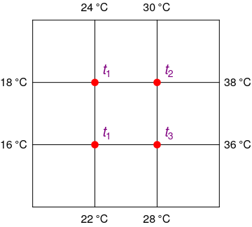
- Sensitivity of solutions
- Linear independence
- Plane transformations
- Space transformations
- Linear transformations
- Affine maps
- Exercises
- Answers
Matrix Algebra
- Introduction
- Manipulation of matrices
- Partitioned matrices
- Block matrices
- Matrix operators
- Determinants
- Cofactors
- Cramer's rule
- Equivalent matrices
- Elimination: A = L U
- PLU factorization
- Reflection
- Givens rotation
- Special matrices
- Exercises
- Answers
Vector Spaces
- Introduction
- Motivation
- Vector spaces
- Bases
- Dimension
- Coordinate systems
- Linear transformations
- Change of basis
- Matrix transformations
- Compositions
- Isomorphisms
- Dual transformations
- Quotient spaces
- Wedge products
- Rotors
Eigenvalues, Eigenvectors
- Introduction
- Characteristic polynomials
- Companion matrix
- Algebraic and geometric multiplicities
- Minimal polynomials
- Eigenspaces
- Where are eigenvalues?
- Eigenvalues of A B and B A
- Generalized eigenvectors
- Similarity
- Diagonalizability
- Self-adjoint operators
- Exercises
- Answers
Euclidean Spaces
- Introduction
- Dot product
- Euclidean space
- Bilinear transformations
- Norm and distance
- Matrix norms
- Dual norms
- Dual transformations
- Examples of transformations
- Orthogonality
- Gram--Schmidt Process
- Orthogonal matrices
- Self-adjoint matrices
- Unitary matrices
- Projection operators
- QR-decomposition
- Least Square Approximation
- Quadratic forms
- Exercises
- Answers
Matrix Decompositions
- Introduction
- 2D decomposition
- Symmetric matrices
- Symmetric matrices
- Pseudoinverse
- URV-decomposition
- LU-decomposition
- QR-decomposition
- Cholesky decomposition
- Schur decomposition
- Positive matrices
- Roots
- Polar factorization
- Spectral decomposition
- CUR decomposition
- Exercises
- Answers
Tensors
- Introduction
- Circles along curves
- TNB frames
- Tensors
- Tensors in ℝ³
- Tensors & Mechanics
- Differential forms
- Calculus
- Answers
Applications
- Introduction
- GPS problem
- Poisson equation
- Graph theory
- Error correcting codes
- Electric circuits
- FSA
- Markov chains
- Cryptography
- Wave-length transfer matrix
- Computer graphics
- Linear Programming
- Hill's determinant
- Fibonacci matrices
- Discrete dynamic systems
- Discrete Fourier transform
- Fast Fourier transform
- Curve fitting
- Answers
Functions of Matrices
- Introduction
- Diagonalization
- Sylvester formula
- The Resolvent method
- Polynomial interpolation
- Positive matrices
- Roots <
- Pseudoinverse
- Exercises
- Answers
Miscellany
- Introduction
- Circles along curves
- TNB frames
- Differential forms
- Calculus
- Vector representations
- Matrix representations
- Change of basis
- Orthonormal Diagonalization
- Generalized inverse
- Differential forms
Preliminaries
- Complex Number Operations
- Sets
- Polynomials
- Polynomials and Matrices
- Computer solves Systems of Linear Equations
- Location of Eigenvalues
- Power Method
- Iterative Method
- Similarity and Diagonalization
Glossary
Reference

This Book is licensed under Creative Commons Attribution-NonCommercial-NoDerivs 3.0 Unported License
Linear Systems
Linear algebra is the study of linear sets of equations and their transformation properties. Linear algebra is central to almost all areas of mathematics.A linear equation in the variables x₁, x₂, … , xn is an equation of the form
Observe that a linear equation does not involve products or roots of variable or any nonlinear function of these variables. All variables occur only to the first power and do not appear as their products.
Let us start with a system of two linear equations with two unknowns, such as
However, we can save 3 multiplications on expense of 1 division if we multiply the first row by 3/2 (a computer does not afraid of using rational numbers). This yields 8 flops (arithmetic operations) to solve the given linear system.
Do you know another option to solve this system of linear equations? Most likely you were taught that substitution will work. Indeed, expressing x from the first equation (with 3 arithmetic operations: 1 subtraction and 2 divisions), we obtain
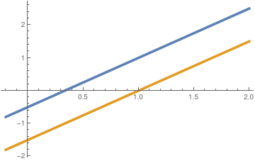
Another option to find the solution is to plot each equation and determine the intersection (if any). Python helps
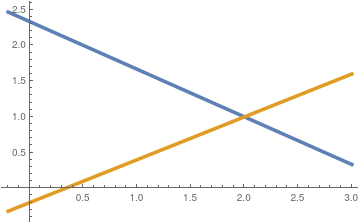
Since every linear equation in two unknowns x and y
|
|
A linear equation in the variables x₁, x₂, … , xn is an equation of the form
Observe that a linear equation does not involve products or roots of variable or any nonlinear function of these variables. All variables occur only to the first power and do not appear as their products.
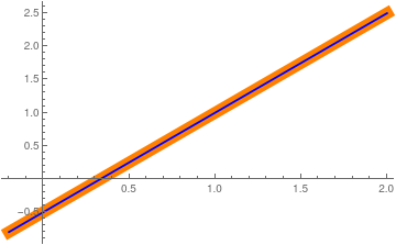
In general, we claim that a linear system of two equations with two unknowns either has a unique solution, or no solution, or infinitely many solutions.
Now we turn our attention to three linear equations in three unknowns:
|
We plot one plane using the equation
\[
a\,x + b\,y + c\,z = a\,x_0 + b\,y_0 + c\, z_0 ,
\]
that passes through the point (x0, y0, z0) and having normal vector (𝑎, b, c).
The following figure shows the case when all three places coicide; then we have infinite many solutions. Next figure shows that there is no solution when two coincident planes parallel to the third; no common intersection.
Next figure shows that there is no solution when two parallel planes crosses the third; no common intersection.
Example 3:
Consider the linear system of equations:
\[
\begin{split}
\phantom{10\,y +}z &= 0,
\\
10\,y -z &= 10 ,
\\
-10\,y -z &= 10 .
\end{split}
\]
Next figure shows that there is no solution. If we substitute z = 0 (from the first equation) into two other equations, we see that they have no common intersection.
Example 4:
Consider the linear system of equations:
\[
\begin{split}
2*x+3\,y -z &= 0,
\\
-3*x+2\,y -z &= 1 ,
\\
4*x -10\,y -z &= 2 .
\end{split}
\]
Next figure shows that there is a unique solution. You will learn shortly how Python can detect this conclusion in a blank of eye.
Example 5:
Consider the linear system of equations:
\[
\begin{split}
\phantom{10\,y +}z &= 0,
\\
10\,y -z &= 0 ,
\\
-10\,y -z &= 0 .
\end{split}
\]
Next figure shows that there are infinitely many solutions. If we substitute z = 0 (from the first equation) into two other equations, we see that they are equivalent.
Example 6:
Consider the linear system of equations:
\[
\begin{split}
\phantom{10\,y +}z &= 0,
\\
10\,y -z &= 0 ,
\\
5\,y -z/2 &= 0 .
\end{split}
\]
We will develop a systematic way to do this for any number of equations with arbitrary number of unknowns (often denoted as x1, x2, x3, …) through the use of matrices and vectors.
A system of linear equations in the variables x1, x2, x3, …, xn is a finite set of m linear equations of
the form
The double subscripting on the coefficients 𝑎i,j of the given coefficients gives their location in the system---the first subscript indicates the equation in which the coefficient occurs, and the second indicates which unknown it multiplies. Foe example, 𝑎2,3 is the second equation and multiplies x3.
\begin{equation} \label{EqLinear.1}
\begin{split}
a_{1,1} x_1 + a_{1,2} x_2 + a_{1,3} x_3 + \cdots + a_{1,n} x_n &= b_1 , \\
a_{2,1} x_1 + a_{2,2} x_2 + a_{2,3} x_3 + \cdots + a_{2,n} x_n &= b_2 , \\
\vdots \qquad\qquad \vdots & \vdots \\
a_{m,1} x_1 + a_{m,2} x_2 + a_{m,3} x_3 + \cdots + a_{m,n} x_n &= b_m .
\end{split}
\end{equation}
A solution to the system of equations above is an ordered n-tuple of numbers s1, s2, s3, …, sn
that is a solution to each of the equations in the system. The set of all possible solutions is
called the solution set of the system \eqref{EqLinear.1}.
A system of linear equations (1) is called consistent if it has at least one solution, and it said to be inconsistent if it has no solution.
A special and important class of systems of linear equations that always have at least one solution is the class of homogeneous equations. These are systems where every bi = 0, i = 1, 2, … , m. One solution to such a system will always be when each variable is 0. This means for a system of two or three variables, the graph of each equation in a homogeneous system passes through the origin.
A system of linear equations (1) is called homogeneous (with accent on "ge") if all terms in right side of Eq.(1) are zeroes,
bi = 0, i = 1, 2, … , m. A system (1) is known as inhomogeneous or nonhomogeneous if at least one entry bi ≠ 0.
Matrix Notation
For a given linear system (1), the matrix A = (𝑎ij), whose (i, j) entry is the coefficient 𝑎ij of the system (1) is called the coefficient matrix:
\[
{\bf A} =\left[ \begin{array}{cccc}
a_{11} & a_{12} & \cdots & a_{1n}
\\
a_{21} & a_{22} & \cdots & a_{2n}
\\
\vdots & \vdots & \ddots & \vdots
\\
a_{m1} & a_{m2} & \cdots & a_{mn}
\end{array}
\right] \quad \mbox{or} \quad {\bf A} =\left( \begin{array}{cccc}
a_{11} & a_{12} & \cdots & a_{1n}
\\
a_{21} & a_{22} & \cdots & a_{2n}
\\
\vdots & \vdots & \ddots & \vdots
\\
a_{m1} & a_{m2} & \cdots & a_{mn}
\end{array}
\right) .
\]
A matrix A whose elements are the coefficients 𝑎ij of a set of simultaneous linear equations (1) to which the column-vector b of right-hand side constant terms of Eq.(1) is appended, is called the augmented matrix. We denote the augmented matrix as
When write an augmented matrix, we will usually drop the vertical line separating the coefficient matrix from the input vector b.
\[
\left( {\bf A}\,\vert\,{\bf b} \right) =
\left( \begin{array}{cccc|c}
a_{11} & a_{12} & \cdots & a_{1n} & b_1
\\
a_{21} & a_{22} & \cdots & a_{2n} & b_2
\\
\vdots & \vdots & \ddots & \vdots & \vdots
\\
a_{m1} & a_{m2} & \cdots & a_{mn} & b_m
\end{array}
\right) , \qquad {\bf b} = \begin{pmatrix} b_1 \\ b_2 \\ \vdots \\ b_m
\end{pmatrix} .
\]

Example 7:
Let us consider the linear system
\[
\begin{split}
2\,x + 3\,y + 4\, z &= 5,
\\
3\,x - 7\,y + 3\,z &= 2,
\\
4\,x + 5\,y - 8\,z &= 3.
\end{split}
\]
The coefficient matrix and the right side vector are
\[
{\bf A} = \begin{bmatrix}
2 & \phantom{-}3 & \phantom{-}4 \\
3 & -7 & \phantom{-}3 \\
4 & \phantom{-}5 & -8
\end{bmatrix} , \qquad {\bf b} = \begin{pmatrix} 5 \\ 2 \\ 3 \end{pmatrix} .
\]
With this in hand, we build the corresponding augmented matrix:
\[
\left( {\bf A}\,|\,{\bf b} \right) = \left( \begin{array}{ccc|c}
2 & \phantom{-}3 & \phantom{-}4 & 5 \\
3 & -7 & \phantom{-}3 & 2 \\
4 & \phantom{-}5 & -8 & 3
\end{array} \right)
\]
|