
Introduction to Linear Algebra
Systems of Linear Equations
- Introduction
- Linear systems
- Vectors
- Linear combinations
- Matrices
- Planes in ℝ³
- Equation A x = b
- Sensitivity of solutions
- Linear independence
- Plane transformations
- Space transformations
- Linear transformations
- Affine maps
- Exercises
- Answers
Matrix Algebra
- Introduction
- Manipulation of matrices
- Partitioned matrices
- Block matrices
- Matrix operators
- Determinants
- Cofactors
- Cramer's rule
- Chiò's method
- Equivalent matrices
- Elimination: A = L U
- PLU factorization
- Reflection
- Givens rotation
- Special matrices
- Exercises
- Answers
Vector Spaces
- Introduction
- Motivation
- Vector spaces
- Bases
- Dimension
- Coordinate systems
- Linear transformations
- Change of basis
- Matrix transformations
- Compositions
- Isomorphisms
- Dual transformations
- Quotient spaces
- Rank
- Solving A x = b
- Exercises
- Answers
Eigenvalues, Eigenvectors
- Introduction
- Characteristic polynomials
- Companion matrix
- Algebraic and geometric multiplicities
- Minimal polynomials
- Eigenspaces
- Where are eigenvalues?
- Eigenvalues of A B and B A
- Generalized eigenvectors
- Similarity
- Diagonalizability
- Self-adjoint operators
- Exercises
- Answers
Euclidean Spaces
- Introduction
- Euclidean space
- Bilinear transformations
- Norm and distance
- Matrix norms
- Dual norms
- Dual transformations
- Examples of transformations
- Orthogonality
- Gram--Schmidt Process
- Orthogonal matrices
- Self-adjoint matrices
- Unitary matrices
- Projection operators
- QR-decomposition
- Least Square Approximation
- Quadratic forms
- Exercises
- Answers
Canonical forms
- Introduction
- 2D decomposition
- 3D decomposition
- Projectors
- Direct-sum decompositions
- Cyclic decompositions
- Symmetric matrices
- Pseudoinverse
- URV-decomposition
- LU-decomposition
- QR-decomposition
- Cholesky decomposition
- Schur decomposition
- Positive matrices
- Roots
- Polar factorization
- Spectral decomposition
- CUR decomposition
- Exercises
- Answers
Applications
- Introduction
- Circles along curves
- TNB frames
- GPS problem
- Coriolis acceleration
- Poisson equation
- Graph theory
- Error correcting codes
- Electric circuits
- FSA
- Markov chains
- Cryptography
- Wave-length transfer matrix
- Computer graphics
- Linear Programming
- Hill's determinant
- Fibonacci matrices
- Discrete dynamic systems
- Discrete Fourier transform
- Fast Fourier transform
- Curve fitting
- Answers
Miscellany
- Introduction
- Circles along curves
- TNB frames
- Differential forms
- Calculus
- Vector representations
- Matrix representations
- Change of basis
- Orthonormal Diagonalization
- Generalized inverse
- Differential forms
Preliminaries
- Complex Number Operations
- Sets
- Polynomials
- Polynomials and Matrices
- Computer solves Systems of Linear Equations
- Location of Eigenvalues
- Power Method
- Iterative Method
- Similarity and Diagonalization
Glossary
Reference

This Book is licensed under Creative Commons Attribution-NonCommercial-NoDerivs 3.0 Unported License
To enhance pedagogical effectiveness, the treatment of the dot product is presented in several distinct sections
We denote by 𝔽 one of the following four fields: ℤ, a set of integers, ℚ, a set of rational numbers, ℝ, a set of real numbers, and ℂ, a set of complex numbers. However, in this section, we mostly use only one of them----the set of real numbers mostly because the definition of length or norm definition involves only ℝ (its extension for ℂ is discussed later in inner product section).
This section is devoted to one of the most important operations in all of linear algebra---dot product. Many operations and algorithms involve dot product, including convolution, correlation, matrix multiplication, duality, the Fourier transform, signal filtering, and many others.
Dot Product
We met many times in previous sections a special linear combination of numerical vectors. For instance, a linear equation in n unknownsRemark 1: Although textbooks on linear algebra define dot product for vectors of the same vector space (mostly because it leads to fruitfully theory and geometric applications), our definition extends the dot product for vectors from different vector spaces, but of the same dimension and over the same field 𝔽 of scalars. Importance of this definition stems from practical applications; for instance, in calculus you learn that the line integral involves definition of the dot product for vector field F with infinitesimal dr:
Let us make a numerical experiment by choosing the following matrices: \[ \mathbf{A}_1 = \begin{bmatrix} 1& 2.1 \\ -3& 2.2 \\ -3& -1.5 \end{bmatrix}, \quad \mathbf{A}_2 = \begin{bmatrix} -4& 1.3 \\ 1& 2.6 \\ 5& -3.1 \end{bmatrix}, \quad \mathbf{A}_3 = \begin{bmatrix} 2& 1.7 \\ 2& 6.2 \\ 8& 3.9 \end{bmatrix} . \] Then their dot product will be \[ \mathbf{a} \bullet \mathbf{b} = \begin{bmatrix} -3.& 10.6 \\ -5.& 18. \\ 9.& -6.8 \end{bmatrix} . \]
Remark 2: In applications, numerical vectors are usually associated with measurements and so inherit units. For instance, integer 5 is associated with 5 millions of dollars in Wall street offices, the same number is considered as a 5 dollars bill by a bank's clerk, but mechanical engineer may look at it as 5 centimeters, and computer science folks consider this information as 5 GB. Only mathematicians see in 5 an integer or number without any unit. Therefore, vectors and scalars in Linear Algebra are not related to any specific unit measurements. Now we all appreciate the beauty of mathematical language because we enter our particular information into a computer---this device recognizes only electric pulses as on or off---there is no room for any unit. When Joseph Fourier (1768--1830) introduced the Fourier transform in 1822
If v represents a displacement (e.g., it has SI units in meters) and f represents a force (e.g., with units in Newtons), then f • v represents a work (in Newton-meters or Joules). Therefore, the force has units of "Joules per meter".
If v represents a velocity (e.g., in meters per second) and φ represents momentum (e.g., in kg/s), then φ(v) = m • v represents kinetic energy (in kg²/s² or Joules). Therefore, the dual vector (momentum) has units of "kg*m/s". ■
Remark 3: Recall that two vector spaces V and U are isomorphic (denoted V ≌ U) if there is a bijective linear map between them. This bijection (which is one-to-one and onto mapping) can be achieved by considering ordered bases α = [ a₁, a₂, … , an ] and β = [ b₁, b₂, … , bn ] in these vector spaces V and U, respectively. Then components of every vector with respect to a chosen ordered basis can be identified uniquely with an n-tuple. Therefore, the algebraic formula \eqref{EqDot.2} is essentially applied to two isomorphic copies of the Cartesian product 𝔽n. Geometric interpretation of the dot product, which is coordinate independent and therefore conveys invariant properties of these products, is given in the Euclidean space section.
Note: The definition of the dot product does not restrict of applying it to two distinct isomorphic versions of the direct product 𝔽n ≅ 𝔽n×1 ≅ 𝔽1×n. It is the basic computational building-block from which many operations and algorithms are built. So you can find the dot product of a row vector with a column vector. However, we try to avoid writing it as matrix multiplication,
When evaluating dot product, Maple does not distinguish rows from columns till some extend. Dot product can be accomplished with two Maple commands: with(LinearAlgebra): a := <1, 2, 3> b := Vector[row]([3, 2, 1] c := Vector([1, -1, 1]); result := DotProduct(a, b); \[ result := 10 \] DotProduct(b, a) \[ 10 \] a . b \[ \begin{bmatrix} 3 & 2 & 1 \\ 6&4& 2 \\ 9&6&3 \end{bmatrix} \] However, b . a \[ 10 \] DotProduct(b, c) \[ 2 \] DotProduct(c, b) \[ 2 \] b . c \[ 2 \] c . c \[ 3 \] But c . b \[ \begin{bmatrix} 3&2&1 \\ -3&-2&-1 \\ 3&2&1 \end{bmatrix} \] As you see, when you specify one vector as a column and another as a row, the order matters when you "dot product" (not Maple comamnd DotProduct): ???????

One of the main and fruitful applications of the dot product is observed when scalar product involves numerical vectors from 𝔽n or their isomorphic copies. Upon introducing an ordered basis α = [e₁, e₂, … , en] in a finite dimensional vector space V, every its vector v = c₁e₁ + c₂e₂ + ⋯ + cnen is uniquely identified with the corresponding coordinate vector ⟦v⟧α = (c₁, c₂, … , cn) ∈ 𝔽n.
a := Vector([2, -3]); b := Vector[row]([5, 4]); result := DotProduct(a, b); # Returns -2 \[ result := -2 \] with(LinearAlgebra)
result := DotProduct(b, a); \[ result := -2 \] You can also evaluate the dot product as multiplication: b . a \[ -2 \]
Calculate the dot product of two three dimensional vectors a = (3, 2, 1) and b = (4, −5, 2).
Solution: Using the component formula (1) for the dot product of three-dimensional vectors \[ \mathbf{a} \bullet \mathbf{b} = a_1 b_1 + a_2 b_2 + a_3 b_3 , \] we calculate the dot product to be \[ \mathbf{a} \bullet \mathbf{b} = 3 \cdot 4 - 2 \cdot 5 + 1 \cdot 2 = 4. \]
Dot[a, b]
Maple uses the command DotProduct for evaluation dot product
a.b
a.b
Not every curvilinear system of coordinates supports dot product, as the following example shows.
Definition of dot product in polar coordinates is presented in section "Dot product in coordinate systems" and Example 23. ■
Properties of dot product
The basic properties (1--4) of the dot product are valid for vectors from the same vector space, but the last one involves compatible vector dimensions. In presented properties, u, v, and w are finite dimensional vectors, and λ is a number (scalar):
- u • u > 0 and u • u = 0 if and only if u = 0.
- u • v = v • u (commutative law);
- (u + v) • w = u • w + v • w (distributive law);
- (λ u) • v = λ (u • v) = u • (λ v) (associative law);
-
for any two column vectors u ∈ ℝn×1, v ∈ ℝm×1, and matrix A ∈ ℝm×n, the following equation holds:
v • Au = ATv • u, where AT (A′) is the transpose of matrix A.
A similar relation holds for row vectors: u • vA = uAT • v.
- This property is trivial because \[ \mathbf{u} \bullet \mathbf{u} = u_1^2 + u_2^2 + \cdots + u_n^2 > 0 \] unless all components of vector u are zeroes.
- Applying the definition of dot product to u · v and v · u, we obtain \begin{align*} \mathbf{u} \bullet \mathbf{v} &= u_1 v_1 + u_2 v_2 + \cdots + u_n v_n \\ \mathbf{v} \bullet \mathbf{u} &= v_1 u_1 + v_2 u_2 + \cdots + v_n u_n \end{align*} Since product of two numbers from field 𝔽 is commutative, we conclude that u · v = v · u.
- Since every finite dimensional vector space is isomorphic to 𝔽n, we can assume that these vectors u, v, and w belong to the direct product 𝔽n. Then \[ \mathbf{u} + \mathbf{v} = \left( u_1 , \ldots , u_n \right) + \left( v_1 , \ldots , v_n \right) = \left( u_1 + v_1 , \ldots , u_n + v_n \right) . \] Taking the dot product with w, we get \begin{align*} \left( \mathbf{u} + \mathbf{v} \right) \bullet \mathbf{w} &= \left( u_1 + v_1 , u_2 + v_2 , \ldots , u_n + v_n \right)\left( w_1 , \ldots , w_n \right) \\ &= u_1 w_1 + v_1 w_1 + \cdots u_n w_n + v_n w_n \\ &= \mathbf{u} \bullet \mathbf{w} + \mathbf{v} \bullet \mathbf{w} . \end{align*}
- The left-hand side is \[ \left( \lambda\,\mathbf{u} \right) \bullet \mathbf{v} = \lambda\,u_1 v_1 + \cdots + \lambda u_n v_n = \lambda \left( u_1 v_1 + \cdots + u_n v_n \right) , \] which equal to the right-hand side λ (u • v).
- For matrix A = [𝑎i,j] ∈ ℝm×n, we have \[ \mathbf{v} \bullet \mathbf{A}\,\mathbf{u} = \sum_{i=1}^m v_i \left( \mathbf{A}\,\mathbf{u} \right)_i \] where the i-th component of A u is \[ \left( \mathbf{A}\,\mathbf{u} \right)_i = \sum_{j=1}^n a_{i.j} u_j . \] Changing the order of summation, we get \begin{align*} \mathbf{v} \bullet \mathbf{A}\,\mathbf{u} &= \sum_{i=1}^m v_i \sum_{j=1}^n a_{i.j} u_j \\ &= \sum_{j=1}^n \sum_{i=1}^m v_i a_{i.j} u_j = \sum_{j=1}^n u_j \left( \mathbf{A}^{\mathrm T} \mathbf{v} \right)_j , \end{align*} which is u • (ATv.
Note that the associative law for scalar product (v • u) • w ≠ v • (u • w) is not valid in general; see the following example.
-
Any nonzero vector will work; for instance, v = (3, −2, 1) ∈ ℝ³. Then
\[
\mathbf{v} \bullet \mathbf{v} = 3^2 + (-2)^2 + 1^2 = 9+4+1 = 14 > 0.
\]
{3, -2, 1} . {3, -2, 1}14
-
Commutativity holds because the dot product is implemented element-
wise, and each element-wise multiplication is simply the product
of two scalars. Scalar multiplication is commutative, and therefore the dot product is commutative.
Let \[ \mathbf{v} = \left( 1, 2, 3 \right) , \quad \mathbf{u} = \left( 4, -6, 5 \right) \in \mathbb{R}^3 . \] Then their scalar product is 7, independently of the order of multiplication,as Mathematica confirms:
v = {1, 2, 3}; u = {4, -6, 5}; v.u7Dot[u, v]7 -
Suppose we need to find a dot product of two numerical vectors v • u, one of which has large entries. For instance,
\[
\mathbf{v} = \begin{pmatrix} 3791 \\ -5688 \\ 2894 \end{pmatrix} , \quad \mathbf{u} = \begin{pmatrix} 3 \\ 2 \\ 4 \end{pmatrix} .
\]
Scalar product of these numerical vectors involves large unpleasant multiplications and summation. Using distributive property, we break vector v into sum of four vectors:
\[
\mathbf{v} = \mathbf{v}_1 + \mathbf{v}_2 + \mathbf{v}_3 + \mathbf{v}_4 ,
\]
where
\[
\mathbf{v}_1 = \begin{pmatrix} 1 \\ -8 \\ 4 \end{pmatrix} , \ \mathbf{v}_2 = \begin{pmatrix} 90 \\ -80 \\ 90 \end{pmatrix} , \ \mathbf{v}_3 = \begin{pmatrix} 700 \\ -600 \\ 800 \end{pmatrix} , \ \mathbf{v}_4 = \begin{pmatrix} 3000 \\ -5000 \\ 2000 \end{pmatrix} .
\]
The corresponding four scalar products are not tedious to find:
u = {3,2,4}; v1 = {1,-8,4}; v2 = {90, -80, 90}; v3 = {700,-600,800}; v4 = {3000,-5000,2000}; d1 = u.v13d2 = u.v2470d3 = u.v34100d4 = u.v47000Adding these four numbers, we get the required dot product: \begin{align*} \mathbf{v} \bullet \mathbf{u} &= \left( \mathbf{v}_1 + \mathbf{v}_2 + \mathbf{v}_3 + \mathbf{v}_4 \right) \bullet \mathbf{u} = \mathbf{v}_1 \bullet \mathbf{u} + \mathbf{v}_2 \bullet \mathbf{u} + \mathbf{v}_3 \bullet \mathbf{u} + \mathbf{v}_4 \bullet \mathbf{u} \\ &= 3+470+4100+7000 = 11573 . \end{align*}d1+d2+d3+d411573
-
We set λ = 3.1415926, v = (236, -718), u = (892, 435). Without computer assistance determination of corresponding dot products will be time consuming. So we ask Mathematica for help and find that
\[
\left( \lambda\mathbf{u} \right) \bullet \mathbf{v} = \lambda \left( \mathbf{u} \bullet \mathbf{v} \right) = \mathbf{u} \bullet \left( \lambda \mathbf{v} \right) \approx 319871.
\]
la =3.1415926; v = {236,-718}; u = {892, 435}; (la*u) . v319871.u . (la*v)319871.la*(v . u)319871.
-
Let us take a singular matrix and two 3-column vectors:
\[
\mathbf{A} = \begin{bmatrix} 1&2&3 \\ 4&5&6 \\ 7&8&9 \end{bmatrix} , \quad \mathbf{u} = \begin{pmatrix} 35 \\ -11 \\ 17 \end{pmatrix} , \quad \mathbf{v} = \begin{pmatrix} 23 \\ 97 \\ 41 \end{pmatrix} .
\]
A = {{1, 2, 3}, {4, 5, 6}, {7,8 ,9}};We set vectors v and u as 3-tuples (elements of ℝ³) but not column vectors (elements of ℝ3×1) because Mathematica is smart to understand that we want column vectors.
u = {35,-11,17}; v = {23,97,41};u = {{35}, {-11}, {17}}; v = {{23}, {97}, {41}};
Dot[u, A . v]25049andDot[Transpose[A] . u, v]25049Now we check the same property for row vectors:Dot[u . A, v]25049Dot[v . Transpose[A], u]25049Rectangular matrix: we consider 3-by-2 matrix \[ \mathbf{A} = \begin{bmatrix} 1&2 \\ 3&4 \\ 5&6 \end{bmatrix} \] and two column vectors \[ \mathbf{u} = \begin{pmatrix} a \\ b \end{pmatrix}, \qquad \mathbf{v} = \begin{pmatrix} c \\ d \\ e \end{pmatrix} . \] Then \[ \mathbf{A}\,\mathbf{u} = \begin{bmatrix} 1&2 \\ 3&4 \\ 5&6 \end{bmatrix}\begin{pmatrix} a \\ b \end{pmatrix} = \begin{pmatrix} 1\cdot a + 2 \cdot b \\ 3 \cdot a + 4 \cdot b \\ 5 \cdot a + 6 \cdot b \end{pmatrix} . \] Its dot product with v becomes \[ \mathbf{v} \bullet \mathbf{A}\,\mathbf{u} = c \left( a + 2\,b \right) + d \left( 3\,a + 4\, b \right) + e \left( 5\,a + 6\, b \right) . \tag{A} \] On the other hand, \[ \mathbf{A}^{\mathrm T} \mathbf{v} = \begin{bmatrix} 1 & 3 & 5 \\ 2&4&6 \end{bmatrix} \begin{pmatrix} c \\ d \\ e \end{pmatrix} = \begin{pmatrix} 1\cdot c + 3\cdot d + 5\cdot e \\ 2 \cdot c + 4 \cdot d + 6 \cdot e \end{pmatrix} . \] Then its dot product with u becomes \[ \mathbf{A}^{\mathrm T} \mathbf{v} \bullet \mathbf{u} = a \left( c + 3\, d + 5\, e \right) + b \left( 2\,c + 4\, d + 6\, e \right) . \tag{B} \] Do you need a computer assistance to check that expression (A) is the same as (B) ? I don't need it.
-
Extra warning:
We demonstrate that the identity v • (u • w) = (v • u) • w is not valid for arbitrary vectors v, u, and w. It is true only when v is a scalar multiple of w. Indeed, let k = u • w and c = v • u. Then
\[
\mathbf{v} \bullet \left( \mathbf{u} \bullet \mathbf{w} \right) = \left( \mathbf{v} \bullet \mathbf{u} \right) \bullet \mathbf{w} \quad \iff \quad \mathbf{v} k = c \mathbf{w} .
\]
from the latter, it follows that vectors v and w are collinear.
We choose three vectors (and write them in column form): \[ \mathbf{v} = \begin{pmatrix} 1 \\ 2 \end{pmatrix} , \quad \mathbf{u} = \begin{pmatrix} 3 \\ 4 \end{pmatrix} , \quad \mathbf{w} = \begin{pmatrix} 5 \\ 6 \end{pmatrix} . \] Then \[ \mathbf{v} \bullet \left( \mathbf{u} \bullet \mathbf{w} \right) = \begin{pmatrix} 1 \\ 2 \end{pmatrix} \cdot 39 = \begin{pmatrix} 39 \\ 78 \end{pmatrix} \]
v = {1, 2}; u = {3, 4}; w = {5, 6};
u . w39v*39{39, 78}and \[ \left( \mathbf{v} \bullet \mathbf{u} \right) \bullet \mathbf{w} = 11 \cdot \begin{pmatrix} 5 \\ 6 \end{pmatrix} = \begin{pmatrix} 55 \\ 66 \end{pmatrix} . \]Dot[v, u]1111*w{55, 66}However, for some vectors, we observe v • (u • w)) = (v • u) • w. Let us pick up three vectors \[ \mathbf{v} = \begin{pmatrix} 1 \\ 2 \end{pmatrix} , \quad \mathbf{u} = \begin{pmatrix} 3 \\ 5 \end{pmatrix} , \quad \mathbf{w} = \begin{pmatrix} 2 \\ 4 \end{pmatrix} . \] Then \[ \mathbf{v} \bullet \left( \mathbf{u} \bullet \mathbf{w} \right) = \mathbf{v} \,26 = 26 \begin{pmatrix} 1 \\ 2 \end{pmatrix} , \]v = {1, 2}; u = {3,5}; w = {2,4}; u.w26and \[ \left( \mathbf{v} \bullet \mathbf{u} \right) \bullet \mathbf{w} = 13 \mathbf{w} = 13 \begin{pmatrix} 2 \\ 4 \end{pmatrix} . \]v.u13Since \[ 26 \begin{pmatrix} 1 \\ 2 \end{pmatrix} = 13 \begin{pmatrix} 2 \\ 4 \end{pmatrix} , \] we conclude that this identity is valid for collinear vectors v, and w, and arbitrary u.
It is convenient to introduce the following notation: ∥v∥² = v • v. Positive square root of this quantity is call the norm in mathematics. Then Cauchy inequality can be rewritten as \[ \left\vert {\bf u} \bullet {\bf v} \right\vert \le \| {\bf u} \| \cdot \| {\bf v} \| , \] Suppose first that either u or v is zero. Then their dot product is zero and the Cauchy inequality holds.
Now suppose that neither u nor v is zero. It follows that ∥u∥ > 0 and ∥v∥ > 0 because the dot product x • x > 0 for any nonzero vector x. We have \begin{align*} 0 &\le \left( \frac{{\bf u}}{\| {\bf u} \|} + \frac{{\bf v}}{\| {\bf v} \|} \right) \bullet \left( \frac{{\bf u}}{\| {\bf u} \|} + \frac{{\bf v}}{\| {\bf v} \|} \right) \\ &= \left( \frac{{\bf u}}{\| {\bf u} \|} \bullet \frac{{\bf u}}{\| {\bf u} \|} \right) + 2 \left( \frac{{\bf u}}{\| {\bf u} \|} \bullet \frac{{\bf v}}{\| {\bf v} \|} \right) + \left( \frac{{\bf v}}{\| {\bf v} \|} \bullet \frac{{\bf v}}{\| {\bf v} \|} \right) \\ &= \frac{1}{\| {\bf u} \|^2} \left( {\bf u} \bullet {\bf u} \right) + \frac{2}{\| {\bf u} \| \cdot \| {\bf v} \|} \left( {\bf u} \bullet {\bf v} \right) + \frac{1}{\| {\bf v} \|^2} \left( {\bf v} \bullet {\bf v} \right) \\ &= \frac{1}{\| {\bf u} \|^2} \, \| {\bf u} \|^2 + 2 \left( \frac{{\bf u}}{\| {\bf u} \|} \bullet \frac{{\bf v}}{\| {\bf v} \|} \right) + \frac{1}{\| {\bf v} \|^2} \, \| {\bf v} \|^2 \\ &= 1 + 2 \left( \frac{{\bf u}}{\| {\bf u} \|} \bullet \frac{{\bf v}}{\| {\bf v} \|} \right) + 1 \end{align*} Hence, −∥u∥ · ∥v∥ ≤ u • v. Similarly, \begin{align*} 0 &\le \left( \frac{{\bf u}}{\| {\bf u} \|} - \frac{{\bf v}}{\| {\bf v} \|} \right) \bullet \left( \frac{{\bf u}}{\| {\bf u} \|} - \frac{{\bf v}}{\| {\bf v} \|} \right) \\ &= \left( \frac{{\bf u}}{\| {\bf u} \|} \bullet \frac{{\bf u}}{\| {\bf u} \|} \right) - 2 \left( \frac{{\bf u}}{\| {\bf u} \|} \bullet \frac{{\bf v}}{\| {\bf v} \|} \right) + \left( \frac{{\bf v}}{\| {\bf v} \|} \bullet \frac{{\bf v}}{\| {\bf v} \|} \right) \\ &= \frac{1}{\| {\bf u} \|^2} \left( {\bf u} \bullet {\bf u} \right) - \frac{2}{\| {\bf u} \| \cdot \| {\bf v} \|} \left( {\bf u} \bullet {\bf v} \right) + \frac{1}{\| {\bf v} \|^2} \left( {\bf v} \bullet {\bf v} \right) \\ &= \frac{1}{\| {\bf u} \|^2} \, \| {\bf u} \|^2 - 2 \left( \frac{{\bf u}}{\| {\bf u} \|} \bullet \frac{{\bf v}}{\| {\bf v} \|} \right) + \frac{1}{\| {\bf v} \|^2} \, \| {\bf v} \|^2 \\ &= 1 - 2 \left( \frac{{\bf u}}{\| {\bf u} \|} \bullet \frac{{\bf v}}{\| {\bf v} \|} \right) + 1 \end{align*} Therefore, u • v ≤ ∥u∥ · ∥v∥. By combining the two inequalities, we obtain the Cauchy inequality.
The case n = 1 is trivially true. When n = 2, Cauchy’s inequality just says \[ \left( a_1 b_1 + a_2 b_2 \right)^2 \leqslant \left( a_1^2 + a_2^2 \right) \left( b_1^2 + b_2^2 \right) . \] Expanding both sides to find the equivalent inequality \[ 0 \leqslant \left( a_1 b_2 \right)^2 - 2 \left( a_1 b_2 a_2 b_1 \right) + \left(a_2 b_1 \right)^2 . \] From the well-known factorization x² − 2xy + y² = ( x − y)² one finds \[ 0 \leqslant \left( a_1 b_2 - a_2 b_1 \right)^2 , \] and the nonnegativity of this term confirms the truth of Cauchy's inequality for n = 2.
Now that we have proved a nontrivial case of Cauchy’s inequality, we are ready to look at the induction step. If we let H(n) stand for the hypothesis that Cauchy’s inequality is valid for n, we need to show that H(2) and H(n) imply H(n + 1). With this plan in mind, we do not need long to think of first applying the hypothesis H(n) and then using H(2) to stitch together the two remaining pieces. Specifically, we have \begin{align*} & \quad a_1 b_1 + a_2 b_2 + \cdots + a_n b_n + a_{n+1} b_{n+1} \\ &= \left( a_1 b_1 + a_2 b_2 + \cdots + a_n b_n \right) + a_{n+1} b_{n+1} \\ & \leqslant \left( a_1^2 + a_2^2 + \cdots + a_n^2 \right)^{1/2} \left( b_1^2 + b_2^2 + \cdots + b_n^2 \right)^{1/2} + a_{n+1} b_{n+1} , \\ & \leqslant \left( a_1^2 + a_2^2 + \cdots + a_n^2 + a_{n+1}^2 \right)^{1/2} \left( b_1^2 + b_2^2 + \cdots + b_n^2 + b_{n+1}^2 \right)^{1/2} \end{align*} where in the first inequality, we used the inductive hypothesis H(n) and in the second inequality we used H(2) in the form \[ \alpha \beta + a_{n+1} b_{n+1} \leqslant \left( \alpha^2 + a_{n+1}^2 \right)^{1/2} \left( \beta^2 + b_{n+1}^2 \right)^{1/2} , \] with the new variables \[ \alpha = \left( a_1^2 + a_2^2 + \cdots + a_n^2 \right)^{1/2} , \quad \beta = \left( b_1^2 + b_2^2 + \cdots + b_n^2 \right) . \]
Now we set vector u to be u = 2.71828 v. Using Mathematica, we repeat all previous calculations for these two vectors.
Equality: We consider two vectors in ℝ²: \[ \mathbf{v} = \left( 1 , 2 \right) , \qquad \mathbf{u} = \left( 2 , 4 \right) \] They are linearly dependent because u = 2v. Their scalar product is \[ \left( 1 , 2 \right) \bullet \left( 2 , 4 \right) = 1 \cdot 2 + 2 \cdot 4 = 10. \] I hope that you can square this number without a computer assistance. Norms squared of these vectors are \[ \| \mathbf{v} \|^2 = 1^2 + 2^2 = 5 , \qquad \| \mathbf{u} \|^2 = 2^2 + 4^2 = 4 + 16 = 20 . \] Their product becomes \[ \| \mathbf{v} \|^2 \cdot \| \mathbf{u} \|^2 = 5 \cdot 20 = 100 = 10^2 = \left( \mathbf{v} \bullet \mathbf{u} \right)^2 . \] ■
Important Note: Cauchy's inequality is not valid for complex vector spaces as the following example shows for two 2-vectors u = (1, j) and v = (1, −j), where j is the imaginary unit vector of the complex plane ℂ so j² = −1.
The inequality \eqref{EqDot.3} is also referred to as the Cauchy--Schwarz or Cauchy--Bunyakovsky--Schwarz or usually as CBS inequality.
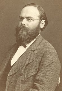
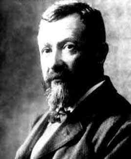
The inequality \eqref{EqDot.3} was first proved by the French mathematician, engineer, and physicist baron Augustin-Louis Cauchy in 1821. In 1859, Victor Bunyakovsky extended this inequality to the case of infinite summation, that is, he established the integral version of the Cauchy inequality. Contribution of Hermann Schwarz (1843--1921) to the Cauchy inequality is unknown neither to me nor to AI except that he married a daughter of the famous mathematician Ernst Eduard Kummer. In 1888, about 30 years after Bunyakovsky's publication, Hermann presented a proof similar to Bunyakovsky's one,
 |
 |
 |
||
|---|---|---|---|---|
| Augustin-Louis Cauchy | Victor Yakovlevich Bunyakovsky | Hermann Amandus Schwarz |
The first step toward the Bunyakovsky result is to establish inequality
Another matrix: We repeat all previous calculations with another not positive definite matrix \[ \mathbf{A} = \begin{bmatrix} -249& -292& -276& 412 \\ 136& 161& 150& -226 \\ 185& 218& 205& -308 \\ 69& 82& 76& -115 \end{bmatrix} . \] Its characteristic polynomial is det(λI − A) = (λ − 1)³(λ + 1). The corresponding dot products are
The following assessment provides a matrix version of Cauchy's inequality. Recall that |·| = det(·) denotes the determinant of a square matrix.
For the remainder of the proof we assume |A ′B| ≠ 0. Using the singular value decomposition we can write A and B as A = P₁D₁Q₁ and B = P₂D₂Q₂, where the m × n matrix Pi and n × n matrix Qi satisfy Pi′Pi = Qi′Qi = In, and Di is an n × n diagonal matrix with positive diagonal elements. It then follows that \[ \left\vert \mathbf{A}^{\mathrm T}\mathbf{B} \right\vert^2 = \left\vert \mathbf{A} \mathbf{Q}'_1 \mathbf{D}_1 \mathbf{P}'_1 \mathbf{P}_2 \mathbf{D}_2 \mathbf{Q}_2 \right\vert^2 = \left\vert \mathbf{D}_1 \right\vert^2 \left\vert \mathbf{D}_2 \right\vert^2 \left\vert \mathbf{P}'_1 \mathbf{P}_2 \right\vert^2 , \] while |A ′A| = |D₁|² and |B ′B| = |D₂|². Hence the conclusion of Theorem 4 follows directly from |P₁′P₁| ≤ 1. Also we have equality if and only if P₁P₁′ = P₂P₂′ , and since this is equivalent to A and B having the same column space; the proof is complete.
Its proof is based on Young’s inequality
Using decomposition Theorem:
Let A and B be m × m symmetric matrices with B being positive definite. Let Λ = diag(λ₁, λ₂, … , λm), where λ₁, λ₂, … , λm are the eigenvalues of B−1A. Then a nonsingular matrix C exists, such that \[ \mathbf{C}\,\mathbf{A}\,\mathbf{C}^{\mathrm T} = \Lambda , \quad \mathbf{C}\,\mathbf{B}\,\mathbf{C}^{\mathrm T} = \mathbf{I}_m . \]
we can write A = T Λ Tt and B = T Tt, where T is a nonsingular matrix, Λ = diag(λ₁, λ₂, … , λn), and λ₁, λ₂, … , λn are the eigenvalues of B−1A, and Tt is transpose matrix. Thus, the proof will be complete if we can show that \[ \left\vert \Lambda \right\vert^{\alpha} = \prod_{i=1}^n \lambda_i^{\alpha} \leqslant \left\vert \alpha \Lambda + \left( 1 - \alpha \right) \mathbf{I}_n \right\vert = \prod_{i=1}^n \left( \alpha \lambda_i + 1 - \alpha \right) , \] with equality if and only if Λ = In. This result is easily confirmed by showing the function g(λ) = αλ + 1 − α − λα is minimized at λ = 1 when 0 ≤ α ≤ 1.
Dot Product and Linear Transformations

The fundamental significance of the dot product is that it is a linear transformation of vectors in each multiplier. This means that the function f(v) = u • v is a linear functional for any fixed vector u. Then scalar product can be defined as a bilinear form:
Metric via Dot Product
In mathematics, a metric space is a set where a notion of distance between any two elements (usually called points) is defined, satisfying specific axioms: non-negativity, identity of indiscernibles, symmetry, and the triangle inequality. Essentially, it's a set with a defined distance function that allows us to measure how "far apart" any two elements are.
A vector space, by definition, has no metric inside it, which is very desirable property. It turns out that the scalar product can be used to define length or distance between vectors transferring ℝn into a metric space, known as the Euclidean space. In order to distinguish metric space from vector space with metric, mathematicians call the magnitude or length of vector v by norm and denote it as ∥v∥.

A first relation between the angles α and β is found if we project the sides AC and BC onto AB \[ c = b\,\cos\alpha + a\,\cos\beta . \] Projecting similarly onto the other sides, we are led to two further equations (which can be obtained from the first one by the use of circular permutations). Here is the system \[ \begin{cases} b\,\cos\alpha + a\,\cos\beta \phantom{+b\,\cos\gamma} &= c , \\ \phantom{b\,\cos\alpha} c \,\cos\beta + b\,\cos\gamma &= a , \\ c\,\cos\alpha + \phantom{c\.\cos\beta} + a\,\cos\gamma &= b . \end{cases} \] It is linear in the three variables x₁ = cosα, x₂ = cosβ, x₃ = cosγ. Let us solve this system by Gaussian elimination: \begin{align*} \left( \begin{array}{ccc|l} b&a&0&c \\ 0&c&b&a \\ c&0&a&b \end{array} \right) &\sim \left( \begin{array}{ccc|l} b&a&0&c \\ 0&c&b&a \\ 0& -\frac{c}{b}\,a & a& b - \frac{c}{b}\,c \end{array} \right) \\ &\sim \left( \begin{array}{ccc|l} b&a&0&c \\ 0&c&b&a \\ 0&0& 2a & b - \frac{c^2}{b} + \frac{a^2}{b} \end{array} \right) \end{align*} This yields
With standard basis in ℝn
We summarize properties of Euclidean norm in the following assesment.
- ∥v∥ > 0 for v ≠ 0 (positivity).
- ∥λv∥ = |λ| ∥v∥ (scaling).
- ∥v + u∥ ≤ ∥v∥ + ∥u∥ (triangle inequality).
- | ∥v∥ − ∥u∥ | ≤ ∥v − u∥ ≤ ∥v∥ + ∥u∥.
- This property follows immediately from the definition \[ \mathbf{v} \bullet \mathbf{v} = v_1^2 + v_2^2 + \cdots + v_n^2 . \] A sum of positive entries cannot be negative, and it is zero only when every term is zero.
- It has been shown previously.
- By definition, \begin{align*} \| \mathbf{v} - \mathbf{u} \|^2 &= \left( \mathbf{v} - \mathbf{u} \right) \bullet \left( \mathbf{v} - \mathbf{u} \right) \\ &= \mathbf{v} \bullet \mathbf{v} + \mathbf{v} \bullet \mathbf{u} + \mathbf{u} \bullet \mathbf{v} + \mathbf{u} \bullet \mathbf{u} = \| \mathbf{v} \|^2 + \| \mathbf{u} \|^2 + 2\,\mathbf{v} \bullet \mathbf{u} . \end{align*} Using Cauchy's inequality, we get \[ \left\vert \mathbf{v} \bullet \mathbf{u} \right\vert \le \| \mathbf{v} \| \cdot \| \mathbf{u} \| . \] This yields \[ \| \mathbf{v} - \mathbf{u} \|^2 \le \| \mathbf{v} \|^2 + \| \mathbf{u} \|^2 + 2\,\| \mathbf{v} \| \cdot \| \mathbf{u} \| = \left( \| \mathbf{v} \| + \| \mathbf{u} \| \right)^2 . \]
- Similarly to the previous proof, \[ \| \mathbf{v} - \mathbf{u} \|^2 = \left( \mathbf{v} - \mathbf{u} \right) \bullet \left( \mathbf{v} - \mathbf{u} \right) = \| \mathbf{v} \|^2 + \| \mathbf{u} \|^2 - 2\left( \mathbf{v} \bullet \mathbf{u} \right) \] Again from Cauchy's inequality, \[ - 2\left( \mathbf{v} \bullet \mathbf{u} \right) \ge 2\,\| \mathbf{v} \| \cdot \| \mathbf{u} \| , \] which leads to \[ \| \mathbf{v} - \mathbf{u} \|^2 \ge \| \mathbf{v} \|^2 + \| \mathbf{u} \|^2 - 2\, \| \mathbf{v} \| \cdot \| \mathbf{u} \| = \left( \| \mathbf{v} \| - \| \mathbf{u} \| \right)^2 . \] The next inequality \( \displaystyle \quad \| \mathbf{v} - \mathbf{u} \| \le \| \mathbf{v} \| + \| \mathbf{u} \| \quad \) follows from the triangle inequality (property 3).
Using Mathematica, we verify properties included in Theorem 6 with the following examples.
- This formulas follows from the identity: \[ \mathbf{v} \bullet \mathbf{v} = v_1^2 + v_2^2 + \cdots + v_n^2 . \] which is zero only when all components of vector v are zeroes.
-
We generate a vector of size five:
v = Flatten[RandomReal[{-1, 1}, {1, 5}]]{0.371645, -0.811594, 0.591386, -0.037053, 0.758338}Upon choosing a real scalar λ = 2.71, we multiply2.71*v{1.00716, -2.19942, 1.60266, -0.100414, 2.0551}Its norm isNorm[2.71*v]3.55722Now we calculate the norm of v and multiply the result by λ = 2.71,2.71*Norm[v]3.55722
-
We generate two vectors of length five:
v = RandomInteger[{-8, 8}, {1, 5}]{{-1, -7, 0, 6, 1}}u = RandomInteger[{-7, 8}, {1, 5}]{{-1, 3, -2, 2, 3}}In order to verify the triangle inequality, we evaluate both sides:N[Norm[u] + Norm[v]]14.5235N[Norm[u + v]]10.198\[ 10.198 \approx \| \mathbf{v} + \mathbf{u} \| < \| \mathbf{v} \| + \| \mathbf{u} \| \approx 14.5235 . \]
-
We choose randomly two vectors
v = Flatten[RandomInteger[{-7, 9}, {1, 6}]]
u = Flatten[RandomInteger[{-7, 9}, {1, 6}]]{5, 9, -5, 1, 2, -2}Their norms are
{-1, -6, 3, -5, -3, -1}Norm[v]2 Sqrt[35]Norm[u]9The difference of norms isN[Norm[v] - Norm[u]]2.83216The norm of their difference isN[Norm[v - u]]19.6723The sum of norms isN[Norm[v] + Norm[u]]20.8322These numbers confirm inequalities in part 4.
Scalar multiplication property allows us to define, for any non-zero vector v ∈ ℝn, an associated normalized vector n with unit length given by

Upon introducing the norm (meaning length or magnitude) of a vector, \( \displaystyle \quad \| {\bf v} \| = +\sqrt{{\bf v} \bullet {\bf v}} , \quad \) Cauchy's inequality can be written as

Using points A(0, 0, c), B(𝑎, 0, 0), and C(0, b, 0), we find vectors \[ \mathbf{u} = \vec{BA} = (-a, 0, c) \qquad\mbox{and} \qquad \mathbf{v} = \vec{BC} = (-a, b, 0) . \] Their norms \[ \| \mathbf{u} \| = \sqrt{a^2 + c^2} , \qquad \|\mathbf{v} \| = \sqrt{a^2 + b^2} \] and dot product \[ \mathbf{u} \bullet \mathbf{v} = a^2 \] show that formula (8) can be written as \[ \frac{\mathbf{u} \bullet \mathbf{v}}{\| \mathbf{u} \| \cdot \| \mathbf{v} \|} = \frac{a^2}{\sqrt{a^2 + c^2}\cdot\sqrt{a^2 + b^2}} = \cos\theta \] because the ratio is definitely less than 1. For instance, if 𝑎 =1, b = 2, and c = 3, we get \[ \cos\theta = \frac{1}{\sqrt{5}\cdot \sqrt{10}} \qquad \Longrightarrow \qquad \theta = \mbox{arctan}\left( \frac{1}{5\sqrt{2}} \right) \approx 0.14049 . \]
Another angle problem: We consider the same cuboid, but now we are going to determine the angle between a diagonal on a face and a diagonal of the cuboid. Upon plotting Figure 16.2, we are after the angle ∠ABD.

Since point D has coordinates (0, b, c), we find vector \( \displaystyle \quad \mathbf{v} = \vec{BD} = \left( -a, b, c \right) . \quad \) Then the dot product of vectors u and v becomes \[ \mathbf{u} \bullet \mathbf{v} = \left( -a, 0, c \right) \bullet \left( -a, b, c \right) = a^2 + c^2 . \] Then formula (8) yields \[ \cos\theta = \frac{\mathbf{u} \bullet \mathbf{v}}{\| \mathbf{u} \| \, \| \mathbf{v} \|} = \frac{a^2 + c^2}{\sqrt{a^2 + c^2}\,\sqrt{a^2 + b^2 + c^2}} . \] Taking inverse cosine function, we find the angle to be \[ \theta = \mbox{arccos} \left( \frac{\sqrt{a^2 + c^2}}{\sqrt{a^2 + b^2 + c^2}} \right) . \] For 𝑎 =1, b = 2, c = 3, we get \[ \theta = \mbox{arccos} \left( \frac{\sqrt{10}}{\sqrt{14}} \right) \approx 0.563943 = 32.3115^{\circ} . \]
Dot product in not standard bases
When ordered basis [e₁, e₂, … , en] in ℝn is not a standard one, the dot product must be modified in order to maintain regular (Euclidean) distance between points or vectors:
If [e¹, e², … , en] is the dual basis, then the inverse of gi,j is the raised-indices metric tensor for the covector space:
Another basis: \[ \beta = \left[ \mathbf{b}_1 , \mathbf{b}_2 \right] = \left[ \mathbf{i} , \mathbf{i} + \mathbf{j} \right] . \] The vector v = (−3, 4) has the following coordinates in basis β: \[ \mathbf{v} = \left( -3, 4 \right) \qquad \Longrightarrow \qquad \left[\!\left[ \mathbf{v} \right]\!\right]_{\beta} = \left( v^1 , v^2 \right) = \left( -7 , 4 \right) \] because \[ \mathbf{v} = -3\mathbf{i} + 4\mathbf{j} = -3\mathbf{i} + 4 \left( \mathbf{i} + \mathbf{j} - \mathbf{i} \right) = -3\mathbf{i} + 4 \left( \mathbf{i} + \mathbf{j} \right) - 4\mathbf{i} . \] Here we used a mathematical trick: add and subtruct the same value. The second component j is replaced by j + i − i = b₂ − i. The dot product in basis β becomes \begin{align*} \mathbf{v} \bullet \mathbf{v} &= g_{1,1} v^1 v^1 + g_{1,2} v^1 v^2 + g_{2,1} v^2 v^1 + g_{2,2} v^2 v^2 \\ &= g_{1,1} \left( -7 \right)^2 + g_{1,2} \left( -7 \right) \left( 4 \right) + g_{2,1} \left( 4 \right) \left( -7 \right) + g_{2,2} \left( 4 \right)^2 \\ &= g_{1,1} 49 - g_{1,2} 28 - g_{2,1} 28 + g_{2,2} 16 . \end{align*} The components of the metric tensor are \begin{align*} g_{1,1} &= \mathbf{b}^1 \bullet \mathbf{b}^1 = \mathbf{i} \bullet \mathbf{i} = 1 , \\ g_{1,2} &= \mathbf{b}^1 \bullet \mathbf{b}^2 = \mathbf{i} \bullet \left( \mathbf{i} + \mathbf{j} \right) = \mathbf{i} \bullet \mathbf{i} + \mathbf{i} \bullet \mathbf{j} = 1 + 0 = 1 , \\ g_{2,1} &= \mathbf{b}^2 \bullet \mathbf{b}^1 = \mathbf{i} \bullet \left( \mathbf{i} + \mathbf{j} \right) = \mathbf{i} \bullet \mathbf{i} + \mathbf{i} \bullet \mathbf{j} = 1 + 0 = 1 , \\ g_{2,2} &= \mathbf{b}^2 \bullet \mathbf{b}^2 = \left( \mathbf{i} + \mathbf{j} \right) \bullet \left( \mathbf{i} + \mathbf{j} \right) = \mathbf{i} \bullet \mathbf{i} + \mathbf{j} \bullet \mathbf{j} = 2 . \end{align*} Using these values, we calculate the dot product \begin{align*} \mathbf{v} \bullet \mathbf{v} &= 49 - 28 - 26 + 2\cdot 16 = 25 . \end{align*}
Applications
Scalar products are intimately associated with a variety of physical concepts. For example, if the vector is mean-centered---the average of all vector elements is subtracted from each element---then the dot product this vector with itself is called variance in statistics. So it provides a measurement of dispersion across a data set.The work done by a force applied at a point serves as a primary example of dot product because the work is defined as the product of the displacement and the component of the force in the direction of displacement (i.e., the projection of the force onto the direction of the displacement). Thus, the component of the force perpendicular to the displacement "does no work." If F is the force (in Newtons) and s is the displacement (in meters), then the work W is by definition equal to
Naturally, other physical quantities can be expressed in such a way. For example, the electrostatic potential energy gained by moving a charge q along a path C in an electric field E is −q∫C E • dr. We may also note that Ampere's law concerning the magnetic field B associated with a current-carrying wire can be written as \[ \oint_C {\bf B} \bullet {\text d}{\bf r} = \mu_0 I , \] where I is the current enclosed by a closed path C traversed in a right-handed sense with respect to the current direction. ■
2D case: we start with flat (ℝ²).
The area of a 2D triangle whose vertices are 𝑎 = (x𝑎, y𝑎), b = (xb, yb), c = (xc, yc) (as shown in figure 1) is given by \[ \mbox{area} = \frac{1}{2} \begin{vmatrix} x_b - x_a & x_c - x_a \\ y_b - y_a & y_c - y_a \end{vmatrix} . \]

Barycentric coordinates allow us to express the coordinates of p = (x, y) in terms of 𝑎, b, c. More specifically, the barycentric coordinates of p are the numbers β and γ such that \[ p = a + \beta\left( b-a \right) + \gamma \left( c -a \right) \] If we regroup 𝑎, b, c, we obtain \begin{align*} p &= a + \beta\,b - \beta\,a + \gamma\,c - \gamma\,a \\ &= \left( a - \beta \right) a + \beta\,b + \gamma\,c . \end{align*} It is customary to define a third variable α by \[ \alpha = 1 - \beta - \gamma . \] Then we have \[ p = \alpha\,a + \beta\, b + \gamma\,c , \qquad \alpha + \beta + \gamma = 1 . \] The barycentric coordinates of the point p in terms of the points 𝑎, b, c are the numbers α, β, γ such that p = α𝑎 + βb + γc, with α + β + γ = 1.
Barycentric coordinate are defined for all points in the plane. They have several nice features:
- A point p is inside the triangle defined by 𝑎, b, c if and only if \[ 0 < \alpha < 1 , \quad 0 < \beta < 1 , \quad 0 < \gamma < 1 . \] This property provides an easy way to test if a point is inside a triangle.
- If one of the barycentric coordinates is 0 and the other two are between 0 and 1, the corresponding point p is on one of the edges of the triangle.
- If any barycentric coordinate is less than zero, then p must lie outside of the triangle.
- If two of the barycentric coordinates are zero and the third is 1, the point p is at one of the vertices of the triangle.
- By changing the values of α, β, γ between 0 and 1, the point p will move smoothly inside the triangle. This can (and will) be applied to other properties of the vertices such as color problem.
- The center of the triangle is obtained when α = β = γ = ⅓. If the triangle is made of a certain substance which is evenly distributed throughout the triangle, then these values of α, β, γ would give us the center of gravity.
Let A𝑎, Ab and Ac be as in figure 1 and let A denote the area of the triangle. Also note that the point inside the triangle on figure 1 is the point we called p. Consider the triangles in the figure. These are different triangles drawn for a fixed value of β. They have the same area since they have the same base and height. This area was denoted Ab on figure 1. Thus, we see that Ab only depends on β. Therefore, we have \[ A_b = C\beta . \] for some constant C. When p is on b that is when β = 1, we have Ab = A. Hence, A = C. Therefore we see that \[ \beta = \frac{A_b}{A} . \] Similarly, we have \[ \alpha = \frac{A_a}{A} , \qquad \gamma = \frac{A_c}{A} . \] In coordinates, these parameters become \[ \beta = \frac{\begin{vmatrix} x_a - x_c & x - x_c \\ y_a - y_c & y - y_c \end{vmatrix}}{\begin{vmatrix} x_b - x_a & x_c - x_a \\ y_b - y_a & y_c - y_a \end{vmatrix}} , \] \[ \gamma = \frac{\begin{vmatrix} x_b - x_a & x - x_a \\ y_b - y_a & y - y_a \end{vmatrix}}{\begin{vmatrix} x_b - x_a & x_c - x_a \\ y_b - y_a & y_c - y_a \end{vmatrix}} , \]
Let us assume that we are using the RGB model. That is all colors can be obtained by mixing R (red), G (green) and B (blue). Usually, with such a model, the level of each color channel is a number between 0 and 255. To specify the color at any point, we must specify a triplet (R, G, B) where R, G, and B are integers between 0 and 255. They indicate how much of red, green and blue is used in the color. When using Java, there is a built-in class to handle colors. It is called Color. This class has some built-in predefined colors. Here are some examples: Color.black, Color.blue, Color.cyan, Color.gray, Color.green, Color.magenta, Color.orange, Color.pink, Color.red, Color,white, Color.yellow. To get any other color, one uses a statement such as new Color(R,G,B) where R,G,B are integers between 0 and 255.
It is also possible to use a single integer to represent colors. Keeping in mind that an integer has 32 bits, bits 0 − 7 contain the R level, bits 8 − 15 contain the G level and bits 16−23 contain the B level. The remaining bits are unused and set to 0. Let us see now how barycentric coordinates can be used to smoothly color a triangle, given the color of its vertices. Using the notation above, let us assume that C𝑎 is the color of 𝑎, Cb is the color of b and Cc is the color of c. Each color is in fact a triplet. We will use the notation C𝑎 = (R𝑎, G𝑎, B𝑎) and similar notation for the remaining points. We would like to color the triangle so that there is a smooth coloring throughout the triangle. We use the fact that by changing the values of α, β, γ between 0 and 1, the point p = α𝑎 + βb + γc will move smoothly inside the triangle. In other words, small changes in α, β, γ will result in small changes in the location of p. We apply this to colors. We let \[ C = \alpha C_a + \beta C_b + \gamma C_c \] (we really do this for every color channel). Small changes in α, β, γ will result in small changes in the color. Therefore, the color will change smoothly as we move within the triangle. To color smoothly a triangle given the color of its vertices, we can use the following algorithm:
- For each point P = (x, y) inside the triangle, find α, β, γ.
- Use α, β, γ to interpolate the color of the point from the color of the vertices using relation \[ C = \alpha C_a + \beta C_b + \gamma C_c \]
- Plot the point with coordinates (x, y) and color computed above.
3D case:
We use the same notation as in the 2D case. The only difference is that now points have three coordinates. So, we have 𝑎 = (x𝑎, y𝑎, z𝑎), b = (xb, yb, zb) and c = (xc, yc, zc). Barycentric coordinates are extended naturally to 3D triangles and they have the same properties. In other words, we have the same equation for point p = α𝑎 + βb + γc.
The only difference of 3D compared to 2D is that the area of the triangle is alwuas positive independently on orientation. We define the following quantities:
- n is the normal to the triangle T with vertices (𝑎, b, c) in counterclockwise order. In other words, n = (b − 𝑎) × (c − 𝑎).
- n𝑎 is the normal to T𝑎, the triangle with area A𝑎 as shown in figure 1. T𝑎 = (b, c, p) in counterclockwise order. Thus, n𝑎 = (c − b) × (p − b).
- nb is the normal to Tb, the triangle with area Ab as shown in figure 1. Tb = (c, 𝑎, p) in counterclockwise order. Thus, nb = (𝑎 − c) × (p − c).
- nc is the normal to Tc, the triangle with area Ac as shown in figure 1. Tc = (𝑎, b, p) in counterclockwise order. Thus, nc = (b − 𝑎) × (p − 𝑎).
Dot product in floating point format
All arithmetic operations performed by computers over floating point numbers are subject to round-off procedure, which is a mapping of real numbers into floating-point numbers. Let fl(x) denote the rounding-off result for x. For instance, fl(π) = 0.31415926 × 10⁻¹. Then
The dot product of two vectors, when calculated with floating-point numbers, can be affected by rounding errors. This is because floating-point arithmetic involves approximations, and repeated multiplication and addition can lead to accumulated errors, especially when dealing with very large or very small numbers (Avogadro's number = 6.023 x 10²³ and Planck's constant = 6.626068 x 10⁻³⁴).
Since x • y does not necessarily have a representation in the floating-point format with bounded mantissa, there is no algorithm which always computes dot-products exactly. Thus, one seeks to construct an algorithm which computes a floating-point number with minimal deviation from the exact result where the deviation should not depend on the number of addends.
Although floating point error analysis done in numerical linear algebra, we consider a simple algorithm for evaluation of the dot product of two vectors x • y:
s = 0;
for i = 1:n
    s = s + x(i)∗y(i);
end
At the first step, we have
Now we apply the triangle inequality (and |δi|, |ϵi| ≤ η) to the difference between the computed and exact values:
We consider two numerical vectors with entries from ℚ4: \[ \mathbf{a} = \left( \frac{3}{7} , \ \frac{2}{5},\ \frac{6}{13} , \ \frac{11}{23} \right) , \quad \mathbf{b} = \left( \frac{7}{15} , \ \frac{5}{12} , \ \frac{23}{47} , \ \frac{5}{11} \right) . \] Their dot product in exact arithmetics is \[ \mathbf{a} \bullet \mathbf{b} = \frac{3481}{4230} \approx 0.8229314420803783 . \]
- Find the dot product of the following pairs of vectors. \[ {\bf (a)\ \ } \begin{pmatrix} 1 \\ -3 \\ 4 \end{pmatrix} , \quad \begin{pmatrix} 8 \\ 6 \\ 1 \end{pmatrix} \qquad {\bf (b)\ \ } \begin{pmatrix} 3 \\ 5 \\ 6 \end{pmatrix} , \quad \begin{pmatrix} -9 \\ 2 \\ 3 \end{pmatrix} \]
- how that for any vectors, x, y ∈ ℝn, we have \[ \| \mathbf{x} + \mathbf{y} \|^2 = \| \mathbf{x} \|^2 + 2\,\mathbf{x} \bullet \mathbf{y} + \| \mathbf{y} \|^2 . \] 𝑥 , 𝑦 ∈ 𝑅 𝑛 , we have
- For vectors u, v ∈ ℝn, show that \( \displaystyle \quad (\mathbf{u} \bullet \mathbf{v}) = \frac{1}{4} \left( \| \mathbf{u} + \mathbf{v} \|^2 - \| \mathbf{u} - \mathbf{v} \|^2 \right) . \)
- Prove the parallelogram identity: \[ \| \mathbf{u} + \mathbf{v} \|^2 + \| \mathbf{u} - \mathbf{v} \|^2 = 2\, \| \mathbf{u} \|^2 + 2\,\| \mathbf{v} \|^2 . \]
- What is the angle between the vectors i + j and i + 3j?
- What is the area of the quadrilateral with vertices at (1, 1), (4, 2), (3, 7) and (2, 3)?
- Find cos(θ) where θ is the angle between the vectors \[ \left( 3, -2, 7 \right) \quad \mbox{and} \quad \left( 5,3,4 \right) . \]
- Find cos(θ) where θ is the angle between the vectors \[ \left( \right) \quad \mbox{and} \quad \left( \right) . \]
- Verify the Cauchy inequality for vectors \[ \left( \right) \quad \mbox{and} \quad \left( \right) . \]
- Find proju(v) where \[ \left( \right) \quad \mbox{and} \quad \left( \right) . \]
- Find proju(v) where \[ \left( \right) \quad \mbox{and} \quad \left( \right) . \]
- Decompose the vector v into v = v∥ + v⊥, where \[ \left( \right) \quad \mbox{and} \quad \left( \right) . \]
- Show that \[ \mathbf{u} \bullet \left( \mathbf{v} - \mbox{proj}_u (\mathbf{v}) \right) = 0 \] and conclude every vector in &Ropf'n can be written as the sum of two vectors, one of which is orthogonal and another is parallel to the given vector.
- Are the vectors u = (2, 3, −1, 4) and v = (?, ?, ?, ?) T orthogonal?
- Aldaz, J. M.; Barza, S.; Fujii, M.; Moslehian, M. S. (2015), "Advances in Operator Cauchy—Schwarz inequalities and their reverses", Annals of Functional Analysis, 6 (3): 275–295, doi:10.15352/afa/06-3-20
- Bunyakovsky, Viktor (1859), "Sur quelques inequalities concernant les intégrales aux différences finies" (PDF), Mem. Acad. Sci. St. Petersbourg, 7 (1): 6
- Cauchy, A.-L. (1821), "Sur les formules qui résultent de l'emploie du signe et sur > ou <, et sur les moyennes entre plusieurs quantités", Cours d'Analyse, 1er Partie: Analyse Algébrique 1821; OEuvres Ser.2 III 373-377
- Deay, T. and Manogue, C.A., he Geometry of the Dot and Cross Products, Journal of Online Mathematics and Its Applications 6.
- Gibbs, J.W. and Wilson, E.B., Vector Analysis: A Text-Book for the Use of Students of Mathematics & Physics: Founded Upon the Lectures of J. W. Gibbs, Nabu Press, 2010.
- Magnus, J. R. (1988). Linear Structures. Charles Griffin, London.
- Marcus, M. & Minc, H. (1992). A Survey of Matrix Theory and Matrix Inequalities. Dover Publications. Corrected reprint of the 1969 edition.
- Schwarz, H. A. (1888), "Über ein Flächen kleinsten Flächeninhalts betreffendes Problem der Variationsrechnung" (PDF), Acta Societatis Scientiarum Fennicae, XV: 318, archived (PDF) from the original on 2022-10-09
- Solomentsev, E. D. (2001) [1994], "Cauchy inequality", Encyclopedia of Mathematics, EMS Press
- Steele, J. M. (2004). The Cauchy–Schwarz Master Class: An Introduction to the Art of Mathematical Inequalities. Cambridge University Press.
- Vector addition