
Introduction to Linear Algebra with Mathematica
Systems of Linear Equations
- Introduction
- Linear systems
- Vectors
- Linear combinations
- Matrices
- Planes in ℝ³
- Row operations
- Gaussian elimination
- Reduced Row-Echelon Form
- Equation A x = b
- Sensitivity of solutions
- Iterative methods
- Linear independence
- Plane transformations
- Space transformations
- Linear transformations
- Affine maps
- Exercises
- Answers
Matrix Algebra
- Introduction
- Manipulation of matrices
- Matrix transformations
- Block matrices
- Determinants
- Cofactors
- Cramer's rule
- Partitioned matrices
- Elementary matrices
- Inverse matrices
- Elimination: A = LU
- PLU factorization
- Reflection
- Givens rotation
- Special matrices
- Exercises
- Answers
Vector Spaces
- Introduction
- Motivation
- Vector spaces
- Bases
- Dimension
- Coordinate systems
- Change of basis
- Linear transformations
- Compositions
- Isomorphisms
- Dual spaces
- Dual transformations
- Subspaces
- Intersections
- Direct sums
- Quotient spaces
- Vector products
- Cross products
- Matrix spaces
- Row space
- Range or Column space
- Rank
- Null Spaces or Kernels
- Dimension Theorems
- Four subspaces
- Solving A x = b
- Exercises
- Answers
Eigenvalues, Eigenvectors
- Introduction
- Characteristic polynomials
- Algebraic and geometric multiplicities
- Minimal polynomials
- Eigenspaces
- Where are eigenvalues?
- Eigenvalues of AB and BA
- Generalized eigenvectors
Euclidean Spaces
- Introduction
- Dot product
- Bilinear transformations
- Inner product
- Norm and distance
- Matrix norms
- Dual norms
- Dual transformations
- Examples of transformations
- Orthogonality
- Gram--Schmidt Process
- Orthogonal sets
- Self-adjoint Matrices
- Unitary matrices
- Projection operators
- QR-decomposition
- Least Square Approximation
- Quadratic forms
- Exercises
- Answers
Matrix Decompositions
- Introduction
- LU-decomposition
- QR-decomposition
- Cholesky decomposition
- Schur decomposition
- Jordan decomposition
- Positive matrices
- Roots
- Polar factorization
- Spectral decomposition
- Singular values
- SVD <
- Pseudoinverse
- Exercises
- Answers
Applications
- GPS Problem
- Graph Theory
- Error Correcting Codes
- Electric Circuits
- Markov Chains
- Cryptography
- Wave-length Transfer Matrix
- Computer Graphics
- Linear Programming
- Hill's Determinant
- Fibonacci Matrices
- Discrete Fourier Transform
- Fast Fourier Transform
- Curve fitting
Functions of Matrices
- Introduction
- Similar matrices
- Diagonalization
- Sylvester Formula
- The Resolvent method
- Polynomial Interpolation
- Positive Matrices
- Roots <
- Pseudoinverse
- Exercises
- Answers
Miscellany
- Circles along curves
- TNB frames
- Tensors I
- Tensors II
- Differential forms
- Calculus
- Vector Representations
- Matrix Representations
- Change of Basis
- Orthonormal Diagonalization
- Generalized Inverse
- Differential forms
Preliminaries
- Complex Number Operations
- Sets
- Polynomials
- Polynomials and Matrices
- Computer solves Systems of Linear Equations
- Location of Eigenvalues
- Power Method
- Iterative Method
- Similarity and Diagonalization
Glossary
Reference

This Book is licensed under Creative Commons Attribution-NonCommercial-NoDerivs 3.0 Unported License
The methods, starting from an initial guess x(0), iteratively apply some formulas to detect the solution of the system. For this reason, these methods are often indicated as iterative methods. In this section, we explore one-step iterative methods that may be beneficial. When applied, they proceed iteratively by successively generating sequences of vectors that approach a solution to a linear system. In many instances (such as when the coefficient matrix is sparse, that is, contains many zero entries), iterative methods can be faster and more accurate than direct methods. Furthermore, the amount of memory required for a sparse coefficient n×n matrix A is proportional to n. Also, iterative methods can be stopped whenever the approximate solution they generate is sufficiently accurate.
Iterative methods
To demonstrate applications of iterative methods in linear algebra, we consider the system of n linear equations with n unknowns x1, x2, … , xn (here n is a positive integer):When a sequence of errors ek = x(k) − c convergences fast enough to zero, iterative methods are competitive with direct methods, which require much more memory and have a higher computational complexity. There are several references on iterative methods to solve a system of linear equations; for example, P.G. Ciarlet, J.J. Dongarra et al., C.T. Kelley, G. Meurant, and Y. Saad.
There are infinite many ways to introduce an equivalent fixed point problem for the given equation (1) or (2). In order to apply an iterative method for solving system of equations (1), or its equivalent compact form (2), we need to rearrange this equation to the fixed point form (3). This can be achieved by splitting the matrix A = S + M, where S is a nonsingular matrix. S is also called a preconditioner, and its choice is crucial in numerical analysis. Then the equation A x = b is the same as S x = b −M x. Application of the inverse matrix S−1 yields the fixed point equation (3), which becomes
- The new vector x(k+1) should be easy to compute. Hence, S should be a simple (and invertible!) matrix; it may be diagonal or triangular.
-
The sequence { x(k) } should converge to the true solution x = c. If we subtract the iteration
in equation (5) from the true equation x = S−1b − S−1M x, the result is a formula involving only the errors ek = c − x(k):
\begin{equation} \label{EqJacobi.6} {\bf e}_{k+1} = - {\bf S}^{-1} {\bf M} \,{\bf e}_k = \left( - {\bf S}^{-1} {\bf M} \right)^{k+1} {\bf e}_0 , \qquad k=0,1,2,\ldots . \end{equation}
If ∥ · ∥ denotes some vector norm (this topic is covered in Part 5 of this tutorial) on
ℝn and
the corresponding of (−S−1M) is less than 1, we claim that x(k) − c → 0 as
k → ∞. Indeed,
The foregoing result holds for any standard norm on ℝn because they all equivalent.
Theorem 1: Let x(0) be an arbitrary vector in ℝn and define x(k+1) = S−1b − S−1M x(k) for k = 0, 1, 2,, …. If x = c is the solution to Eq.(4), then a necessary and sufficient condition for x(k) → c is that all eigenvalues of matrix S−1M be less than 1, i.e., | λ | < 1.
In other words, the iterative method in equation (5) is convergent if and only if every eigenvalue of S−1M satisfies | λ | < 1. Its rate of convergence depends on the maximum size of eigenvalues of matrix S−1M. So the largest eigenvalue will eventually be dominant.
.
The Jacobi method
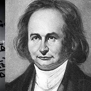
In numerical linear algebra, the Jacobi method (a.k.a. the Jacobi iteration method) is an iterative algorithm for determining the solutions of a strictly diagonally dominant system of linear equations. Each diagonal element is solved for, and an approximate value is plugged in. The method was discovered by Carl Gustav Jacob Jacobi in 1845.
The idea of this iteration method is to extract the main diagonal of the matrix of the given vector equation
Here is the algorithm for Jacobi iteration method:
Input: initial guess x(0) to the solution, (diagonal dominant) matrix A, right-hand side
       vector b, convergence criterion
Output: solution when convergence is reached
Comments: pseudocode based on the element-based formula above

k = 0
while convergence not reached do
    for i := 1 step until n do
        σ = 0
        for j := 1 step until n do
            if j ≠ i then
                σ = σ + aij xj(k)
            end
        end
        xi(k+1) = (bi − σ) / aii
    end
    increment k
end
Jacobi's method begins with solving the first equation for x₁ and the second equation for x₂, to obtain
| n | 0 | 1 | 2 | 3 | 4 | 5 |
|---|---|---|---|---|---|---|
| x₁ | 0 | \( \displaystyle \frac{7}{6} \) | \( \displaystyle \frac{22}{21} \approx 1.04762 \) | \( \displaystyle \frac{101}{63} \approx 1.60317 \) | \( \displaystyle \frac{682}{441} \approx 1.54649 \) | \( \displaystyle \frac{2396}{1323} \approx 1.81104 \) |
| x₂ | 0 | \( \displaystyle -\frac{1}{7} \) | \( \displaystyle \frac{11}{21} \approx 0.52381 \) | \( \displaystyle \frac{67}{147} \approx 0.455782 \) | \( \displaystyle \frac{341}{441} \approx 0.773243 \) | \( \displaystyle \frac{2287}{3087} \approx 0.740849 \) |
The successive vectors \( \displaystyle \quad \begin{bmatrix} x_1^{(k)} \\ x_2^{(k)} \end{bmatrix} \quad \) are called iterates. For instance, when k = 5, the fifth iterate is \( \displaystyle \quad \begin{bmatrix} 1.8110 \\ 0.740849 \end{bmatrix} \quad \)
Here is Python code to produce the result you see above, first using a module, which is used in other examples also.
the 47th iteration: [2. 0.99999998]
the 48th iteration: [1.99999998 1. ]
the 49th iteration: [2. 0.99999999]
the 50th iteration: [1.99999999 1. ]
In code above, parameter n_ is for the number of iterations you want - the display is always the last 5 iterations; fp_ is for floating point, the default being "True" - if you input "False" as the last argument, you will get explicit solution, which produces fractions when input coefficients are from ℚ.
| Matrix | A | Λ | L | U | b | x0 |
|---|---|---|---|---|---|---|
| \( \displaystyle \begin{pmatrix} 6 & -5 \\ 4 & -7 \end{pmatrix} \) | \( \displaystyle \begin{pmatrix} 6 & 0 \\ 0 & -7 \end{pmatrix} \) | \( \displaystyle \begin{pmatrix} 0&0 \\ 4&0 \end{pmatrix} \) | \( \displaystyle \begin{pmatrix} 0&-5 \\ 0&0 \end{pmatrix} \) | \( \displaystyle \begin{pmatrix} 7 \\ 1 \end{pmatrix} \) | \( \displaystyle \begin{pmatrix} 0 \\ 0 \end{pmatrix} \) | |
| Iterations | 0 | 1 | 2 | 3 | 4 | 5 |
| \( \displaystyle \begin{pmatrix} 0&0 \end{pmatrix} \) | \( \displaystyle \begin{pmatrix} \frac{7}{6} & -\frac{1}{7} \end{pmatrix} \) | \( \displaystyle \begin{pmatrix} \frac{22}{21} & \frac{11}{21} \end{pmatrix} \) | \( \displaystyle \begin{pmatrix} \frac{101}{63} & \frac{67}{147} \end{pmatrix} \) | \( \displaystyle \begin{pmatrix} \frac{682}{441} & \frac{341}{441} \end{pmatrix} \) | \( \displaystyle \begin{pmatrix} \frac{2396}{1323} & \frac{2287}{3087} \end{pmatrix} \) |
Now we repeat calculations by making 50 iterative steps.
N[%]
Expressing the rational numbers above as floating point reals, we get the same result, which is more suitable for human eyes. So, we repeat calculations using floating point representation.
Finally, we can obtain the same result as floating point, also in less than a second.
| Matrix | A | Λ | L | U | b | x0 |
|---|---|---|---|---|---|---|
| \( \displaystyle \begin{pmatrix} 6 & -5 \\ 4 & -7 \end{pmatrix} \) | \( \displaystyle \begin{pmatrix} 6 & 0 \\ 0 & -7 \end{pmatrix} \) | \( \displaystyle \begin{pmatrix} 0&0 \\ 4&0 \end{pmatrix} \) | \( \displaystyle \begin{pmatrix} 0&-5 \\ 0&0 \end{pmatrix} \) | \( \displaystyle \begin{pmatrix} 7 \\ 1 \end{pmatrix} \) | \( \displaystyle \begin{pmatrix} 0 \\ 0 \end{pmatrix} \) | |
| Iterations | 0 | 46 | 47 | 48 | 49 | 50 |
| (2., 1.) | (2., 1.) | (2., 1.) | (2., 1.) | (2., 1.) | (2., 1.) |
Here are the component parts of the code above, producing the same output in steps.
d = DiagonalMatrix[Diagonal[A]];
l = LowerTriangularize[A, -1];
u = UpperTriangularize[A, 1];
b = ({ {7}, {1} });
x[1] = ({ {0}, {0}Sdemo3 });
Grid[{{"A", "d", "l", "u", "b", "x0"}, MatrixForm[#] & /@ {A, d, l, u, b, x[1]}}, Frame -> All]
Starting point does not matter for final destination of Jacobi's ietrating scheme. Let's test that with calculations using different starting points, random floating point numbers and integers. Below, a function is provided that works with a list of starting points.
varSt = MapThread[ Last[Prepend[ FoldList[LinearSolve[d, -(l + u) . # + b] &, {#1, #2}, Range[50]], {"x1", "x2"}]] &,(*starting point->*)stPts][[All, All, 1]];
TableForm[ Transpose[{stPts[[1]], varSt[[All, 1]], stPts[[2]], varSt[[All, 2]]}], TableHeadings -> {None, {"Starting\npoint", "\n\!\(\*SubscriptBox[\(x\), \(1\)]\)", "Starting\npoint", "\n\!\(\*SubscriptBox[\(x\), \(2\)]\)"}}]
| Starting | Starting | ||
|---|---|---|---|
| Point | x₁ | Point | x₂ |
| 0 | 2. | 0 | 1. |
| 0.5 | 2. | 0.5 | 1. |
| 0.25 | 2. | 0.25 | 1. |
| 0.0013514 | 2. | 0.742626 | 1. |
| 10 | 2. | 16 | 1. |
N[Eigenvalues[A]]
| n | 0 | 1 | 2 | 3 | 4 | 5 |
|---|---|---|---|---|---|---|
| x₁ | 0 | \( \displaystyle \frac{4}{5} \) | \( \displaystyle \frac{11}{5} = 2.2 \) | \( \displaystyle \frac{13}{25} = 0.52 \) | \( \displaystyle -\frac{341}{50} = -6.82 \) | \( \displaystyle -\frac{823}{250} = -3.292 \) |
| x₂ | 0 | \( \displaystyle -\frac{5}{2} \) | \( \displaystyle \frac{11}{10} =1.1 \) | \( \displaystyle -\frac{127}{20} = -6.35 \) | \( \displaystyle -\frac{341}{100} = -3.41 \) | \( \displaystyle \frac{2887}{200} = -14.435 \) |
It is hard to believe that this iteration scheme provides the correct answer: x₁ = 2 and x₂ = 1.
the 49th iteration: [-6.49298361e+07 -1.89378693e+08]
the 50th iteration: [-2.27254431e+08 -1.13627216e+08]
the 51th iteration: [-1.36352658e+08 -3.97695257e+08]
the 52th iteration: [-4.77234308e+08 -2.38617154e+08]
the 53th iteration: [-2.86340584e+08 -8.35160041e+08]
b = {4, 10};
LinearSolve[A, b]
Here are the last five runs:
| Matrix | A | Λ | L | U | b | x0 |
|---|---|---|---|---|---|---|
| \( \displaystyle \begin{pmatrix} 5 & -6 \\ 7 & -4 \end{pmatrix} \) | \( \displaystyle \begin{pmatrix} 5 & 0 \\ 0 & -4 \end{pmatrix} \) | \( \displaystyle \begin{pmatrix} 0&0 \\ 7&0 \end{pmatrix} \) | \( \displaystyle \begin{pmatrix} 0&-6 \\ 0&0 \end{pmatrix} \) | \( \displaystyle \begin{pmatrix} 4 \\ 10 \end{pmatrix} \) | \( \displaystyle \begin{pmatrix} 0 \\ 0 \end{pmatrix} \) | |
| Iterations | 48 | 49 | 50 | 51 | 52 | 53 |
| \( \displaystyle \left\{ \begin{array}{c} -1.08216 \times 10^8 , \\ -5.41082 \times 10^7 \end{array} \right\} \) | \( \displaystyle \{ \begin{array}{c} -6.49298 \times 10^7 , \\ -1.89379 \times 10^8 \end{array} \} \) | \( \displaystyle \left\{ \begin{array}{c} -2.27254 \times 10^8 , \\ -3.97695 \times 10^8 \end{array} \right\} \) | \( \displaystyle \{ \begin{array}{c}-4.77234 \times 10^8 , \\ -2.38617 \times 10^8 \end{array} \} \) | \( \displaystyle \left\{ \begin{array}{c} -2.86341 \times 10^8 , \\ -8.3516 \times 10^8 \end{array} \right\} \) | \( \displaystyle \left\{ \begin{array}{c} -2.86341 \times 10^8 , \\ -8.3516 \times 10^8 \end{array} \right\} \) |
To start an iteration method, you need an initial guess vector
|
\begin{equation} \label{EqJacobi.7}
{\bf x}^{(k+1)}_j = \frac{1}{a_{j,j}} \left( b_j - \sum_{i\ne j} a_{j,i} x_i^{(k)} \right) , \qquad j=1,2,\ldots , n.
\end{equation}
|
|---|
If the diagonal elements of matrix A are much larger than the off-diagonal elements, the entries of B should all be small and the Jacobi iteration should converge. We introduce a very important definition that reflects diagonally dominant property of a matrix.
Theorem 2: If a system of n linear equations in n variables has a strictly diagonally dominant coefficient matrix, then it has a unique solution and both the Jacobi and the Gauss--Seidel method converge to it.
b = {5, 21, -9};
LinearSolve[A, b]
However, the code above will not work if you define vector b as column vector. To overcome this, use the following modification.
LinearSolve[A, b][[All,1]]
Upon extracting the diagonal matrix from A, we split the given system (3.1) into the following form: \[ \left( \Lambda + {\bf M} \right) {\bf x} = {\bf b} \qquad \iff \qquad {\bf x} = \Lambda^{-1} {\bf b} - \Lambda^{-1} {\bf M} \,{\bf x} , \] where \[ {\bf d} = \Lambda^{-1} {\bf b} = \begin{bmatrix} \frac{1}{5} & 0 & 0 \\ 0 & \frac{1}{7} & 0 \\ 0 & 0 & \frac{1}{8} \end{bmatrix} \begin{pmatrix} \phantom{-}5 \\ 21 \\ -9 \end{pmatrix} = \begin{bmatrix} 1 \\ 3 \\ - \frac{9}{8} \end{bmatrix} , \qquad {\bf B} = - \Lambda^{-1} {\bf M} = \begin{bmatrix} 0 & \frac{4}{5} & - \frac{1}{5} \\ - \frac{5}{7} & 0 & \frac{4}{7} \\ - \frac{3}{8} & \frac{7}{8} & 0 \end{bmatrix} . \] Matrix B has one real eigenvalue λ₁ ≈ -0.362726, and two complex conjugate eigenvalues λ₂ ≈ 0.181363 + 0.308393j, λ₃ ≈ 0.181363 - 0.308393j, where j is the imaginary unit of the complex plane ℂ, so j² = −1.
Eigenvalues[B]
Although we know exact solution, x₁ = 2, x₂ = 1, x₃ = −1, of the given system of linear equations (3.1), we know that convergence of Jacobi's iteration scheme does not depend on the initial guess. So we start with zero: \[ {\bf x}^{(0)} = \left[ 0, 0, 0 \right] . \]
MatrixForm[%]/
MatrixForm[%]
B= {{0, 4/5, -1/5},{-5/7,0,4/7},{-3/8,7/8,0}};
x2 = d + B.d
B= {{0, 4/5, -1/5},{-5/7,0,4/7},{-3/8,7/8,0}};
x3 = d + B.x2
| Matrix | A | Λ | L | U | b | x0 |
|---|---|---|---|---|---|---|
| \( \displaystyle \begin{pmatrix} 5 & -4 & 1 \\ 5 & 7 & -4 \\ 3 & -7 & 8 \end{pmatrix} \) | \( \displaystyle \begin{pmatrix} 5 & 0& 0 \\ 0 & 7&0 \\ 0&0& 8 \end{pmatrix} \) | \( \displaystyle \begin{pmatrix} 0&0&0 \\ 5&0&0 \\ 3& -7 & 0 \end{pmatrix} \) | \( \displaystyle \begin{pmatrix} 0&-4 & 1 \\ 0&0& -4 \\ 0&0&0 \end{pmatrix} \) | \( \displaystyle \begin{pmatrix} 5 \\ 21 \\ -9 \end{pmatrix} \) | \( \displaystyle \begin{pmatrix} 0 \\ 0 \\ 0 \end{pmatrix} \) | |
| Iterations | 0 | 1 | 2 | 3 | 4 | 5 |
| \( \displaystyle \begin{pmatrix} 0&0&0 \end{pmatrix} \) | \( \displaystyle \begin{pmatrix} 1 & 3 & - \frac{9}{8} \end{pmatrix} \) | \( \displaystyle \begin{pmatrix} \frac{29}{8} & \frac{23}{14} & \frac{9}{8} \end{pmatrix} \) | \( \displaystyle \begin{pmatrix} \frac{117}{56} & \frac{59}{56} & -\frac{67}{64} \end{pmatrix} \) | \( \displaystyle \begin{pmatrix} \frac{4597}{2240} & \frac{713}{784} & -\frac{221}{224} \end{pmatrix} \) | \( \displaystyle \begin{pmatrix} \frac{15091}{7840} & \frac{3043}{3136} & -\frac{2813}{2560} \end{pmatrix} \) |
We repeat calculations with floating point output.
| Matrix | A | Λ | L | U | b | x0 |
|---|---|---|---|---|---|---|
| \( \displaystyle \begin{pmatrix} 5 & -4 & 1 \\ 5 & 7 & -4 \\ 3 & -7 & 8 \end{pmatrix} \) | \( \displaystyle \begin{pmatrix} 5 & 0& 0 \\ 0 & 7&0 \\ 0&0& 8 \end{pmatrix} \) | \( \displaystyle \begin{pmatrix} 0&0&0 \\ 5&0&0 \\ 3& -7 & 0 \end{pmatrix} \) | \( \displaystyle \begin{pmatrix} 0&-4 & 1 \\ 0&0& -4 \\ 0&0&0 \end{pmatrix} \) | \( \displaystyle \begin{pmatrix} 5 \\ 21 \\ -9 \end{pmatrix} \) | \( \displaystyle \begin{pmatrix} 0 \\ 0 \\ 0 \end{pmatrix} \) | |
| Iterations | 0 | 1 | 2 | 3 | 4 | 5 |
| \( \displaystyle \begin{pmatrix} 0&0&0 \end{pmatrix} \) | \( \displaystyle \begin{array}{c} 1. \\ 3. \\ - 1.125 \end{array} \) | \( \displaystyle \begin{array}{c} 3.625, \\ 1.64286, \\ 1.125 \end{array} \) | \( \displaystyle \begin{array}{c} 2.08929, \\ 1.05357, \\ -1.04688 \end{array} \) | \( \displaystyle \begin{array}{c} 2.05223, \\ 0.909439, \\ -0.986607 \end{array} \) | \( \displaystyle \begin{array}{c} 1.92487, \\ 0.970344, \\ -1.09883 \end{array} \) |
We repeat calculations with 20 runs, displaying only the initial and last five:
| Matrix | A | Λ | L | U | b | x0 |
|---|---|---|---|---|---|---|
| \( \displaystyle \begin{pmatrix} 5 & -4 & 1 \\ 5 & 7 & -4 \\ 3 & -7 & 8 \end{pmatrix} \) | \( \displaystyle \begin{pmatrix} 5 & 0& 0 \\ 0 & 7&0 \\ 0&0& 8 \end{pmatrix} \) | \( \displaystyle \begin{pmatrix} 0&0&0 \\ 5&0&0 \\ 3& -7 & 0 \end{pmatrix} \) | \( \displaystyle \begin{pmatrix} 0&-4 & 1 \\ 0&0& -4 \\ 0&0&0 \end{pmatrix} \) | \( \displaystyle \begin{pmatrix} 5 \\ 21 \\ -9 \end{pmatrix} \) | \( \displaystyle \begin{pmatrix} 0 \\ 0 \\ 0 \end{pmatrix} \) | |
| Iterations | 0 | 16 | 17 | 18 | 19 | 20 |
| \( \displaystyle \begin{pmatrix} 0&0&0 \end{pmatrix} \) | (2., 1., −1.) | (2., 1., −1.) | (2., 1., −1.) | (2., 1., −1.) | (2., 1., −1.) |
Theorem 3: If the Jacobi or the Gauss-Seidel method converges for a system of n linear equations in n unknowns, then it must converge to the solution of the system.
Convergence means that "as iterations increase, the values of the iterates get closer and closer to a limiting value:' This means that x(k) converge to r, As usual, we denote by x = c the true solution of the system A x = b.
We must show that r = c. Recall that the Jacobi's (GS is similar) iterates satisfy the equation \[ \Lambda\,{\bf x}^{(k+1)} = {\bf b} + \left( \Lambda - {\bf A} \right) {\bf x}^{(k)} , \qquad k=0,,2,\ldots . \tag{P3.1} \] The Gauss-Seidel method leads to a similar equation where A is further decomposed into upper and lower triangular parts. Application of limit to both sides of Eq.(P3.1), we obtain \[ \Lambda\,{\bf r} = {\bf b} + \left( \Lambda - {\bf A} \right) {\bf r} \qquad \iff \qquad {\bf 0} = {\bf b} - {\bf A}\,{\bf r} . \] Therefore, vector \( \displaystyle {\bf r} = \lim_{k\to \infty} {\bf x}^{(k)} \) satisfies the equation A x = b, so it must be equal to c.
MatrixRank[A]
NullSpace[A]
diag = {{9, 0, 0, 0}, {0, 8, 0, 0}, {0, 0, 7, 0}, {0, 0, 0, 6}};
M = A - diag;
Inverse[diag] . {9, 7, -11, 9}
M = A - diag ;
d = {1, 7/8, -(11/7), 3/2}; B = -Inverse[diag] . M ;
x1 = d + B . d
| n | 0 | 1 | 2 | 3 | 4 | 5 | 10 |
|---|---|---|---|---|---|---|---|
| x₁ | 0 | \( \displaystyle 1 \) | \( \displaystyle \frac{209}{63} \approx 3.31746 \) | \( \displaystyle \frac{40}{189} \approx 0.21164 \) | \( \displaystyle \approx 2.054 \) | \( \displaystyle \approx 2.34034 \) | \( \displaystyle \approx 2.31208 \) |
| x₂ | 0 | \( \displaystyle \frac{7}{8} \) | \( \displaystyle -\frac{89}{112} \approx -0.794643 \) | \( \displaystyle \frac{175}{288} \approx 0.607639 \) | \( \displaystyle \approx 0.305567 \) | \( \displaystyle \approx -0.427675 \) | \( \displaystyle \approx -0.128371 \) |
| x₃ | 0 | \( \displaystyle -\frac{11}{7} \) | \( \displaystyle \frac{1}{2} = 0.5 \) | \( \displaystyle -\frac{1235}{1764} \approx -0.700113 \) | \( \displaystyle \approx -0.922808 \) | \( \displaystyle \approx 0.262426 \) | \( \displaystyle \approx -0.257853 \) |
| x₄ | 0 | \( \displaystyle \frac{3}{2} \) | \( \displaystyle \frac{37}{84} \approx 0.440476 \) | \( \displaystyle \frac{425}{1512} \approx 0.281085 \) | \( \displaystyle \approx 1.25112 \) | \( \displaystyle \approx 0.250038 \) | \( \displaystyle \approx 0.729597 \) |
We are going to make a numerical experiment and check whether Jacobi's iteration depends on the initial guess, which we take closer to the true values: x(0) = [1.5, 0.5, 2.5, 3.5]. Using iteration (4.3), we calculate Jacobi's approximants.
| n | 0 | 1 | 2 | 3 | 4 | 5 | 10 |
|---|---|---|---|---|---|---|---|
| x₁ | 1.5 | 1.61111 | 2.16138 | 1.84245 | 1.84634 | 2.09821 | 1.99034 |
| x₂ | 0.5 | 0.9375 | 0.731647 | 0.810433 | 0.906534 | 0.738926 | 0.815846 |
| x₃ | 2.5 | 2.14286 | 2.35317 | 2.355912.35591 | 2.18519 | 2.37932 | 2.2872 |
| x₄ | 3.5 | 3.41667 | 3.37368 | 3.22828 | 3.3894 | 3.3099 | 3.35227 |
Mathematica confirms these calculations.
This table of iterative values shows that the first coordinate plays around true value x₁ = 2, but we cannot claim convergence of other coordinates, except probably x₂ = 1.
| Matrix | A | Λ | L | U | b | x0 |
|---|---|---|---|---|---|---|
| \( \displaystyle \begin{pmatrix} 9 & -8 & 5&4 \\ 1 & 8 & -5&3 \\ =2 & -4 & 7&-6 \\ 2&-4&-5&6 \end{pmatrix} \) | \( \displaystyle \begin{pmatrix} 9 & 0& 0&0 \\ 0 & 8&0&0 \\ 0&0& 7&0 \\ 0&0&0&6 \end{pmatrix} \) | \( \displaystyle \begin{pmatrix} 0 & 0 & 0&0 \\ 1 & 0 & 0&0 \\ =2 & -4 & 0&0 \\ 2&-4&-5&0 \end{pmatrix} \) | \( \displaystyle \begin{pmatrix} 0 & -8 & 5&4 \\ 0 & 0 & -5&3 \\ 0 & 0 & 0&-6 \\ 0&0&0&0 \end{pmatrix} \) | \( \displaystyle \begin{pmatrix} 9 \\ 7 \\ -11 \\ 9 \end{pmatrix} \) | \( \displaystyle \begin{pmatrix} 0 \\ 0 \\ 0 \\ 0\end{pmatrix} \) | |
| Iterations | 0 | 46 | 47 | 48 | 49 | 50 |
| (0, 0, 0, 0) | {1.67103, 0.131896, -0.455655, 0.651516} |
{1.65994, 0.137018, -0.46018, 0.651207} |
{1.66687, 0.135692, -0.460686, 0.654547} |
{1.66746, 0.133257, -0.4566, 0.650932} |
{1.66142, 0.137093, -0.460923, 0.652518} |
Input: square matrix A and vector b
n is the size of A and vector b
    whle precision condition  do
       for i=1 : n do
           s=0
	   for j=1 : n do
	       if j ≠ i then
	   s = s + 𝑎i,jxj
	       endif
	   endfor
	   yi = (bi−s)/𝑎i,i
	endfor
	   x=y
endwhile
Gauss--Seidel method

Philipp Ludwig von Seidel worked in analysis, probability theory, astronomy, and optics. Unfortunately, he suffered from eye problems and retired at a young age. The paper in which he described the method now known as Gauss Seidel was published in 1874.
The Gauss-Seidel method, which is a modification of the Jacobi algorithm, uses each new value as soon as it is available. This method is based on splitting the matrix A of Eq.(2) into three parts:
Inverse[S]
Inverse[S]
Although structure of the inverse to the lower triangular matrix S = Λ + L can be written explicitly, its practical implementation becomes problematic with size of matrix growth. The n × n matrix S−1 contains n divisions, and its entries contain alternated series, which could be a nightmare for numerical evaluations.
Instead of standard approach (5), the Gauss--Seidel method suggests to extract the strictly lower triangular matrix from S,
Now we demonstrate the iterative procedure above in more detail by showing step by step its application for solving the system of linear equations (2). The first coordinate of x(k+1) is given by Jacobi's formula
|
\begin{equation} \label{EqSeidel.8}
x_j^{(k+1)} = \frac{1}{a_{j,j}} \left( b_j - \sum_{i=1}^{j-1} a_{j,i} x_i^{(k+1)} - \sum_{i=j+1}^n a_{1,i} x_i^{(k)} \right) .
\end{equation}
|
|---|
It is interesting to compare the Jacobi and Gauss–Seidel iterations noting that the latter is using the coordinates of x(k+1) as soon as they are calculated rather than in the next iteration. The program for the Gauss–Seidel iteration is actually simpler than the program for the Jacobi iteration. The vectors x(k) and x(k+1) are both stored in the same vector, x. As a coordinate of x(k+1) is calculated, it replaces the corresponding coordinate of x(k).
Here is algorithm for Gauss-Seidel iteration scheme:
algorithm Gauss–Seidel method is
    inputs: A, b
    output: φ

    Choose an initial guess φ to the solution
    repeat until convergence
        for i from 1 until n do
            σ ← 0
            for j from 1 until n do
                if j ≠ i then
                    σ ← σ + 𝑎i,jφj
                end if
            end (j-loop)
            φi ← (bi − σ) / 𝑎i,i
        end (i-loop)
        check if convergence is reached
end (repeat
input A and b
n is the size of A
while precision conditions do
   for i = 1 : n do
      s = 0
      for j = 1 : n do
         if j ≠ i then
             s = s + 𝑎i,j xj
         end if
      end for
      xi = (1/𝑎i,i) (bi − s)
    end for
end while
b = {12, 4, 14}; LinearSolve[A, b]
If you use column vector b instead of row vector, LinearSolve command should be applied as follows.
Jacobi's algorithm requires extraction of the diagonal matrix A = λ + M, where \[ {\bf A} = \begin{bmatrix} \phantom{-}4 & 2 & -2 \\ -2 & 5 & \phantom{-}2 \\ \phantom{-}4 & 3 & -2 \end{bmatrix} , \qquad \Lambda = \begin{bmatrix} 4 & 0 & \phantom{-}0 \\ 0 & 5 & \phantom{-}0 \\ 0 & 0 & -2 \end{bmatrix} , \quad {\bf M} = \begin{bmatrix} \phantom{-}0 & 2 & -2 \\ -2 & 0 & \phantom{-}2 \\ \phantom{-}4 & 3 & \phantom{-}0 \end{bmatrix} . \]
diag = DiagonalMatrix[{4, 5, -2}]
B = -Inverse[diag] . M
Upon choosing the initial guess to be zero, we obtain the first approximation to be \[ {\bf x}^{(1)} = {\bf d} = \begin{pmatrix} 3 \\ \frac{4}{5} \\ -7 \end{pmatrix} . \] The second iteration step yields \[ {\bf x}^{(2)} = {\bf d} + {\bf B}\,{\bf x}^{(1)} = \begin{pmatrix} - \frac{9}{10} \\ \frac{24}{5} \\ \frac{1}{5} \end{pmatrix} = \begin{pmatrix} -0.9 \\ 4.8 \\ 0.2 \end{pmatrix} . \]
x2 = d + B . d
| Matrix | A | Λ | L | U | b | x0 |
|---|---|---|---|---|---|---|
| \( \displaystyle \begin{pmatrix} 4 & 2 & -2 \\ -2 & 5 & 2 \\ 4 & 3 & -2 \end{pmatrix} \) | \( \displaystyle \begin{pmatrix} 4 & 0& 0 \\ 0 & 5&0 \\ 0&0& -2 \end{pmatrix} \) | \( \displaystyle \begin{pmatrix} 0&0&0 \\ -2&0&0 \\ 4& 3 & 0 \end{pmatrix} \) | \( \displaystyle \begin{pmatrix} 0&2 & -2 \\ 0&0& 2 \\ 0&0&0 \end{pmatrix} \) | \( \displaystyle \begin{pmatrix} 12 \\ 4 \\ 14 \end{pmatrix} \) | \( \displaystyle \begin{pmatrix} 0 \\ 0 \\ 0 \end{pmatrix} \) | |
| Iterations | 0 | 1 | 2 | 3 | 4 | 5 |
| \( \displaystyle \begin{pmatrix} 0&0&0 \end{pmatrix} \) | \( \displaystyle \left( 3, \ \frac{4}{5}, \ -7 \right) \) | \( \displaystyle \left( -\frac{9}{10}, \ \frac{24}{5},\ \frac{1}{5} \right) \) | \( \displaystyle \left( \frac{7}{10},\ \frac{9}{25},\ -\frac{8}{5} \right) \) | \( \displaystyle \left( \frac{101}{50},\ \frac{43}{25},\ -\frac{253}{50} \right) \) | \( \displaystyle \left( -\frac{39}{100},\ \frac{454}{125}, \ -\frac{19}{50} \right) \) |
The errors of Jacobi's iterations at 50-th run are \[ \left\vert x_1^{(50)} -1 \right\vert = 0.039291 , \qquad \left\vert x_2^{(50)} -2 \right\vert = 0.0101124 , \qquad \left\vert x_3^{(50)} +2 \right\vert = 0.069383 . \]
We repeat calculations with 50 runs. It took less than a second to execute the code.
| Matrix | A | Λ | L | U | b | x0 |
|---|---|---|---|---|---|---|
| \( \displaystyle \begin{pmatrix} 4 & 2 & -2 \\ -2 & 5 & 2 \\ 4 & 3 & -2 \end{pmatrix} \) | \( \displaystyle \begin{pmatrix} 4 & 0& 0 \\ 0 & 5&0 \\ 0&0& -2 \end{pmatrix} \) | \( \displaystyle \begin{pmatrix} 0&0&0 \\ -2&0&0 \\ 4& 3 & 0 \end{pmatrix} \) | \( \displaystyle \begin{pmatrix} 0&2 & -2 \\ 0&0& 2 \\ 0&0&0 \end{pmatrix} \) | \( \displaystyle \begin{pmatrix} 12 \\ 4 \\ 14 \end{pmatrix} \) | \( \displaystyle \begin{pmatrix} 0 \\ 0 \\ 0 \end{pmatrix} \) | |
| Iterations | 45 | 46 | 47 | 48 | 49 | 50 |
| {0.950528, 2.01566, -2.08244} |
{0.95095, 2.01319, -2.07545} |
{0.955682, 2.01056, -2.07832} |
{0.95556, 2.0136, -2.0728} |
{0.956802, 2.01134, -2.06848} |
{0.960089, 2.01011, -2.06938} |
Now we apply the Gauss--Seidel method with the same initial choice---the origin. At the first step, we have \begin{align*} x_1^{(1)} &= 3 - \frac{1}{2}\, x_2^{(0)} + \frac{1}{2}\, x_3^{(0)} = 3, \\ x_2^{(1)} &= \frac{4}{5} + \frac{2}{5}\, x_1^{(1)} - \frac{2}{5}\, x_3^{(0)} = 2 \\ x_3^{(1)} &= -7 + 2\,x_1^{(1)} + \frac{3}{2}\,x_2^{(1)} = 2 . \end{align*} Next iteration gives \begin{align*} x_1^{(2)} &= 3 - \frac{1}{2}\, x_2^{(1)} + \frac{1}{2}\, x_3^{(1)} = 3, \\ x_2^{(2)} &= \frac{4}{5} + \frac{2}{5}\, x_1^{(2)} - \frac{2}{5}\, x_3^{(1)} = \frac{6}{5} , \\ x_3^{(2)} &= -7 + 2\,x_1^{(2)} + \frac{3}{2}\,x_2^{(2)} = \frac{4}{5} \end{align*} We manually repeat a few iterations before application of looping procedure. \begin{align*} x_1^{(3)} &= 3 - \frac{1}{2}\, x_2^{(2)} + \frac{1}{2}\, x_3^{(2)} = \frac{14}{5} , \\ x_2^{(3)} &= \frac{4}{5} + \frac{2}{5}\, x_1^{(3)} - \frac{2}{5}\, x_3^{(2)} = \frac{8}{5} , \\ x_3^{(3)} &= -7 + 2\,x_1^{(3)} + \frac{3}{2}\,x_2^{(3)} = 1 , \end{align*} and \begin{align*} x_1^{(4)} &= 3 - \frac{1}{2}\, x_2^{(3)} + \frac{1}{2}\, x_3^{(3)} = \frac{27}{10} , \\ x_2^{(4)} &= \frac{4}{5} + \frac{2}{5}\, x_1^{(3)} - \frac{2}{5}\, x_3^{(3)} = \frac{37}{25} , \\ x_3^{(4)} &= -7 + 2\,x_1^{(4)} + \frac{3}{2}\,x_2^{(4)} = \frac{31}{50} ; \end{align*} \begin{align*} x_1^{(5)} &= 3 - \frac{1}{2}\, x_2^{(4)} + \frac{1}{2}\, x_3^{(4)} = \frac{257}{100} = 2.57 , \\ x_2^{(5)} &= \frac{4}{5} + \frac{2}{5}\, x_1^{(5)} - \frac{2}{5}\, x_3^{(4)} = \frac{79}{50} = 1.58 , \\ x_3^{(5)} &= -7 + 2\,x_1^{(5)} + \frac{3}{2}\,x_2^{(5)} = \frac{51}{100} = 0.51 . \end{align*} Sequential iterates are generated with the following Mathematica code:
| Matrix | A | Λ | L | U | b | x0 |
|---|---|---|---|---|---|---|
| \( \displaystyle \begin{pmatrix} 4 & 2 & -2 \\ -2 & 5 & 2 \\ 4&3&-2 \end{pmatrix} \) | \( \displaystyle \begin{pmatrix} 4 & 0&0 \\ 0 & 5&0 \\ 0&0& -2 \end{pmatrix} \) | \( \displaystyle \begin{pmatrix} 0&0&0 \\ -2&0&0 \\ 4&3&0 \end{pmatrix} \) | \( \displaystyle \begin{pmatrix} 0&2&-2 \\ 0&0&2 \\ 0&0&0 \end{pmatrix} \) | \( \displaystyle \begin{pmatrix} 12 \\ 4 \\ 14 \end{pmatrix} \) | \( \displaystyle \begin{pmatrix} 0 \\ 0 \\ 0 \end{pmatrix} \) | |
| Iterations | 0 | 1 | 2 | 3 | 4 | 5 |
| {0, 0, 0} | \( \displaystyle \left\{ 3, \ 2,\ 2 \right\} \) | \( \displaystyle \left\{ 3,\ \frac{6}{5},\ \frac{4}{5} \right\} \) | \( \displaystyle \left\{ \frac{!4}{5},\ \frac{8}{5}, \ 1 \right\} \) | \( \displaystyle \left\{ \frac{27}{10},\ \frac{37}{25},\ \frac{31}{50} \right\} \) | \( \displaystyle \left\{ \frac{257}{100},\ \frac{79}{50},\ \frac{51}{100} \right\} \) |
We repeat GS-iterative procedure with 50 runs. It tAkes less than a second to execute 50 runs.
| Matrix | A | Λ | L | U | b | x0 |
|---|---|---|---|---|---|---|
| \( \displaystyle \begin{pmatrix} 4 & 2 & -2 \\ -2 & 5 & 2 \\ 4&3&-2 \end{pmatrix} \) | \( \displaystyle \begin{pmatrix} 4 & 0&0 \\ 0 & 5&0 \\ 0&0& -2 \end{pmatrix} \) | \( \displaystyle \begin{pmatrix} 0&0&0 \\ -2&0&0 \\ 4&3&0 \end{pmatrix} \) | \( \displaystyle \begin{pmatrix} 0&2&-2 \\ 0&0&2 \\ 0&0&0 \end{pmatrix} \) | \( \displaystyle \begin{pmatrix} 12 \\ 4 \\ 14 \end{pmatrix} \) | \( \displaystyle \begin{pmatrix} 0 \\ 0 \\ 0 \end{pmatrix} \) | |
| Iterations | 45 | 46 | 47 | 48 | 49 | 50 |
| {1.08661, 1.97577, -1.86312} |
1.08055, 1.97747, -1.87269} |
{1.07492, 1.97904, -1.88159} |
{1.06968, 1.98051, -1.88987} |
The errors of the Gauss--Seidel iterations at 50-th run are \[ \left\vert x_1^{(50)} -1 \right\vert = 0.0602767 , \qquad \left\vert x_2^{(50)} -2 \right\vert = 0.0181273 , \qquad \left\vert x_3^{(50)} +2 \right\vert = 0.095263 . \] As a result of this numerical experiment we conclude that both methods, Jacobi and GS, are very fast and provide approximately the same accuracy, but Jacobi's iteration scheme gives slightly better approximation. Also, a usage of floating foint instead of exact operations with rational numbers does not effect the time of execution.
| Matrix | A | Λ | L | U | b | x0 |
|---|---|---|---|---|---|---|
| \( \displaystyle \begin{pmatrix} 5 & -4 & 1 \\ 5 & 7 & -4 \\ 3&-7&8 \end{pmatrix} \) | \( \displaystyle \begin{pmatrix} 5 & 0&0 \\ 0 &7&0 \\ 0&0& 8 \end{pmatrix} \) | \( \displaystyle \begin{pmatrix} 0&0&0 \\ 5&0&0 \\ 3&-7&0 \end{pmatrix} \) | \( \displaystyle \begin{pmatrix} 0&-4&1 \\ 0&0&-4 \\ 0&0&0 \end{pmatrix} \) | \( \displaystyle \begin{pmatrix} 5 \\ 21 \\ -9 \end{pmatrix} \) | \( \displaystyle \begin{pmatrix} 0 \\ 0 \\ 0 \end{pmatrix} \) | |
| Iterations | 0 | 1 | 2 | 3 | 4 | 5 |
| {0, 0, 0} | \( \displaystyle \left\{ 1, \ 3,\ -\frac{9}{8} \right\} \) | \( \displaystyle \left\{ \frac{29}{8},\ \frac{23}{14},\ \frac{9}{8} \right\} \) | \( \displaystyle \left\{ \frac{!17}{56},\ \frac{59}{56}, \ -\frac{67}{64} \right\} \) | \( \displaystyle \left\{ \frac{4597}{2240},\ \frac{713}{784},\ -\frac{221}{224} \right\} \) | \( \displaystyle \left\{ \frac{15091}{7840},\ \frac{3043}{3136},\ -\frac{2813}{2560} \right\} \) |
We repeat calculations with floating point arithmetic for 50 runs.
| Matrix | A | Λ | L | U | b | x0 |
|---|---|---|---|---|---|---|
| \( \displaystyle \begin{pmatrix} 5 & -4 & 1 \\ 5 & 7 & -4 \\ 3&-7&8 \end{pmatrix} \) | \( \displaystyle \begin{pmatrix} 5 & 0&0 \\ 0 &7&0 \\ 0&0& 8 \end{pmatrix} \) | \( \displaystyle \begin{pmatrix} 0&0&0 \\ 5&0&0 \\ 3&-7&0 \end{pmatrix} \) | \( \displaystyle \begin{pmatrix} 0&-4&1 \\ 0&0&-4 \\ 0&0&0 \end{pmatrix} \) | \( \displaystyle \begin{pmatrix} 5 \\ 21 \\ -9 \end{pmatrix} \) | \( \displaystyle \begin{pmatrix} 0 \\ 0 \\ 0 \end{pmatrix} \) | |
| Iterations | 0 | 46 | 47 | 48 | 49 | 50 |
| {1.86139, 1.25743, -0.722772} |
{1.86139, 1.25743, -0.722772} |
{1.86139, 1.25743, -0.722772} |
{1.86139, 1.25743, -0.722772} |
{1.86139, 1.25743, -0.722772} |
1.86139, 1.25743, -0.722772} |
This example shows that the Gauss--Seidel method converges very slowly: after 50 runs it gives the answer with about 25% accuracy. So Jacobi's method performs much better.
U =U = {{0, -8, 5, -4}, {0, 0, -5, 3}, {0, 0, 0, -6}, {0, 0, 0, 0}} {{0, -8, 5, -4}, {0, 0, -5, 3}, {0, 0, 0, -6}, {0, 0, 0, 0}};
L = A - U
Eq.(6.3) is used to generate Gauss-Seidel iteration: \[ {\bf x}^{(k+1)} = {\bf L}^{-1} {\bf b} - {\bf L}^{-1} {\bf U}\,{\bf x}^{(k)} \qquad \iff \qquad {\bf x}^{(k+1)} = {\bf d} + {\bf B}\,{\bf x}^{(k)} , \qquad k=0,1,2,\ldots . \tag{6.4} \]
Matrix B has rank 3 and all its eigenvalues are real numbers: λ₁ = 1, λ₂ = 0, λ₃ ≈ -0.874609, λ₄ ≈ 0.181487. Therefore, we do not expect convergence of Gauss-Seidel iterations.
| n | 0 | 1 | 2 | 3 | 4 | 5 | 10 |
|---|---|---|---|---|---|---|---|
| x₁ | 0 | 1 | \( \displaystyle \frac{485}{189} \approx 2.56614 \) | 0.925058 | 2.31112 | 1.08992 | 1.94983 |
| x₂ | 0 | \( \displaystyle -\frac{3}{4} \) | \( \displaystyle -\frac{64}{189} \approx -0.338624 \) | 0.534972 | -0.243334 | 0.434793 | -0.0439163 |
| x₃ | 0 | \( \displaystyle -\frac{6}{7} \) | \( \displaystyle -\frac{95}{441} \approx -0.21542 \) | -0.291808 | -0.291808 | -0.733657 | -0.422114 |
| x₄ | 0 | \( \displaystyle \frac{20}{21} \) | \( \displaystyle \frac{950}{3969} \approx .239355 \) | 0.88474 | 0.324231 | 0.815174 | 0.469016 |
Running GS-iterations 50 times yields
| Matrix | A | Λ | L | U | b | x0 |
|---|---|---|---|---|---|---|
| \( \displaystyle \begin{pmatrix} 9 & -8 & 5& -4 \\ 1 & 8 & -5 &3 \\ -2&-4&7 & -6 \\ 2 & -4 &-5& 6 \\ 2& -4& -5& 6 \end{pmatrix} \) | \( \displaystyle \begin{pmatrix} 9 & 0&0&0 \\ 0 &8&0 &0 \\ 0&0& 7& 0 \\ 0&0&0&6 \end{pmatrix} \) | \( \displaystyle \begin{pmatrix} 0&0&0&0 \\ 1&0&0&0 \\ -2&-4&0&0 \\ 2& -4& -5&0 \end{pmatrix} \) | \( \displaystyle \begin{pmatrix} 0&-8&5&-4 \\ 0&0&-5&3 \\ 0&0&0&-6 \\ 0&0&0&0 \end{pmatrix} \) | \( \displaystyle \begin{pmatrix} 9 \\ 7 \\ -11 \\ 9 \end{pmatrix} \) | \( \displaystyle \begin{pmatrix} 0 \\ 0 \\ 0 \\ 0 \end{pmatrix} \) | |
| Iterations | 0 | 46 | 47 | 48 | 49 | 50 |
| {1.65594, 0.119593, -0.528556, 0.587284} |
{1.66096, 0.116801, -0.526738, 0.585265} |
{1.65657, 0.119243, -0.528328, 0.587031} |
{1.66041, 0.117107, -0.526937, 0.585486} |
{1.65705, 0.118975, -0.528154, 0.586837} |
{1.65999, 0.117341, -0.52709, 0.585656} |
Therefore, we conclude that except the first coordinates, all other entries do not converge.
The following table presents Gauss--Seidel iterations with different initial guess.
| n | 0 | 1 | 2 | 3 | 4 | 5 | 10 |
|---|---|---|---|---|---|---|---|
| x₁ | 1.5 | 1.61111 | 2.0751 | 1.81082 | 2.06765 | 1.84769 | 2.00357 |
| x₂ | 0.5 | 0.923611 | 0.778807 | 0.946414 | 0.807257 | 0.930314 | 0.843734 |
| x₃ | 2.5 | 2.41667 | 2.54586 | 2.44308 | 2.53482 | 2.45492 | 2.51133 |
| x₄ | 3.5 | 3.59259 | 3.44905 | 3.56324 | 3.46131 | 3.550083.55008 | 3.48741 |
We repeat calculations with floating point arithmetic for 50 runs.
Successive overrelaxation or SOR method
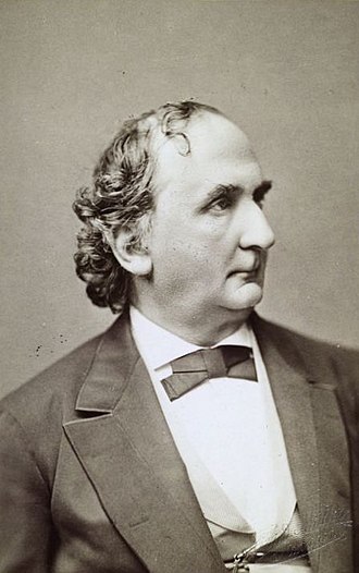
In numerical linear algebra, the method of successive over-relaxation (SOR) is a variant of the Gauss–Seidel method for solving a linear system of equations, resulting in faster convergence. It was devised simultaneously by David M. Young Jr. (1923--2008) and by Stanley P. Frankel (1919--1978) in 1950 for the purpose of automatically solving linear systems on digital computers.When SOR method is applied to the traditional fixed point equation (3), it generates a sequence of approximations according to the formula
To describe application of the overrelaxation for solving system of linear equations (1) or (2), we follow Gauss-Seidel approach and decompose matrix A of coefficients into sum of three matrices:
Inputs: A, b, ω
Output: φ

Choose an initial guess φ to the solution
repeat until convergence
    for i from 1 until n do
        set σ to 0
        for j from 1 until n do
            if j ≠ i then
                set σ to σ + 𝑎i,j φj
            end if
        end (j-loop)
        set φi to (1 − ω)φi + ω(bi − σ) / 𝑎i,i
    end (i-loop)
    check if convergence is reached
end (repeat)
input A and b
input ω
n is the size of A
while precision conditions do
   for i = 1 : n do
      s = 0
      for j = 1 : n do
         if j ne; i then
            s = s + 𝑎i,j xj
         end if
       end for
       xi = ω (bi − s)/ 𝑎i,i + (1 − ω ) xi
    end for
end while
function [x,r,k]=RM(A,b,Omega,kmax,eps1)
% kmax maximum number of iterations;
% eps1 given tolerance;
% Omega: relaxation parameter
% stopping criteria: norm(r)/norm(b)<=eps1 or k>kmax
% Output: x the kth iterate, r the kth residual
% k the number of iterations
% Initial guess is x=0; r=b
n=length(b);r=b;x=zeros(n,1);nb=norm(b);
E=tril(A,-1);D=diag(diag(A));M=(1/Omega)*D-E;
k=1;mr=1;mx=1;e=1;
while e>eps1 & k<=kmax
      dx=M\r;
      x=x+dx;% saxpy operation
      r=r-A*dx;% GAXPY operation
      e=norm(r)/nb;
      k=k+1;
end
Theorem 4 (Kahan, 1958): A necessary condition for the SOR method to converge is ω ∈ (0, 2).
| n | 0 | 1 | 2 | 3 | 4 | 5 |
|---|---|---|---|---|---|---|
| x₁ | 0 | \( \displaystyle \frac{}{} \) | \( \displaystyle \frac{}{} \approx \) | \( \displaystyle \frac{1}{} \approx \) | \( \displaystyle \frac{}{} \approx \) | \( \displaystyle \frac{}{} \approx \) |
| x₂ | 0 | \( \displaystyle -\frac{1}{} \) | \( \displaystyle \frac{}{} \approx \) | \( \displaystyle \frac{}{} \approx \) | \( \displaystyle \frac{}{} \approx \) | \( \displaystyle \frac{}{} \approx \) |
| x₃ | 0 | \( \displaystyle -\frac{1}{} \) | \( \displaystyle \frac{}{} \approx \) | \( \displaystyle \frac{}{} \approx \) | \( \displaystyle \frac{}{} \approx \) | \( \displaystyle \frac{}{} \approx \) |
| x₄ | 0 | \( \displaystyle -\frac{1}{} \) | \( \displaystyle \frac{}{} \approx \) | \( \displaystyle \frac{}{} \approx \) | \( \displaystyle \frac{}{} \approx \) | \( \displaystyle \frac{}{} \approx \) |
diag = DiagonalMatrix[{4, 4, 5}];
B = Inverse[diag] . (A - diag)
| n | 0 | 1 | 2 | 3 | 4 | 5 |
|---|---|---|---|---|---|---|
| x₁ | 0 | \( \displaystyle \frac{}{} \) | \( \displaystyle \frac{}{} \approx \) | \( \displaystyle \frac{1}{} \approx \) | \( \displaystyle \frac{}{} \approx \) | \( \displaystyle \frac{}{} \approx \) |
| x₂ | 0 | \( \displaystyle -\frac{1}{} \) | \( \displaystyle \frac{}{} \approx \) | \( \displaystyle \frac{}{} \approx \) | \( \displaystyle \frac{}{} \approx \) | \( \displaystyle \frac{}{} \approx \) |
| x₃ | 0 | \( \displaystyle -\frac{1}{} \) | \( \displaystyle \frac{}{} \approx \) | \( \displaystyle \frac{}{} \approx \) | \( \displaystyle \frac{}{} \approx \) | \( \displaystyle \frac{}{} \approx \) |
- Let \[ {\bf A} = \begin{bmatrix} 5 & 1 \\ 2 & 6 \end{bmatrix} , \qquad {\bf b} = \begin{bmatrix} \phantom{-}2 \\ -16 \end{bmatrix} , \qquad {\bf x}^{(0)} = \begin{bmatrix} 0 \\ 0 \end{bmatrix} . \] Use Jacobi iteration to compute x(1) and x(2).
- In this exercise, you will see that the order of the equations in a system can affect the performance of an iterative solution method. Upon swapping the order of equations in the previous exercise, we get \[ \begin{split} 2\,x_1 + 6\, x_2 &= -16 , \\ 5\, x_1 + x_2 &= 2 . \end{split} \] Compute five iterations with both the Jacobi and Gauss--Seidel methods using zero as an initial guess.
- Show that if a 2 x 2 coefficient matrix \[ {\bf A} = \begin{bmatrix} a_{1,1} & a_{1,2} \\ a_{2,1} & a_{2,2} \end{bmatrix} \] is strictly diagonally dominant, then the eigenvalues of the iteration matrices B corresponding to the Jacobi and Gauss-Seidel methods are of magnitude < 1 (which guarantees convergence of iteration methods).
- Apply Jacobi's iteration scheme to the system \[ \begin{split} x_1 + x_2 & = 0 , \\ x_1 - x_2 &= 2 . \end{split} \] Do you think that the iteration method converges to the true solution x₁ = 1, x₂ = −1?
- Apply Jacobi's iteration scheme for solving \[ \begin{bmatrix} 2 & 1 \\ 2 & 3 \end{bmatrix} \begin{pmatrix} x_1 \\ x_2 \end{pmatrix} = \begin{pmatrix} \phantom{-}1 \\ -1 \end{pmatrix} . \] Recall that norm of the error is ∥e(k)∥ = ∥B e(k-1)∥ = |λmax| ∥e(k-1)∥, where λmax is the largest (in magnitude) eigenvalue of iteration matrix B. In general (for larger systems), this approximate relationship often is not the case for the first few iterations). Show that the error for this system tends to zero.
- Use the SOR method to solve the system \[ \begin{bmatrix} 2 & 1 \\ 3 & 4 \end{bmatrix} \begin{pmatrix} x_1 \\ x_2 \end{pmatrix} = \begin{pmatrix} \phantom{-}1 \\ -1 \end{pmatrix} . \]
- In the previous exercise, find the characteristic equation for the corresponding matrix B depending on parameter ω. What are its eigenvalues?
- Solve the system of equations with a direct method: \[ \begin{cases} 5 x - 2 y + 3 z &= 8, \\ 3 x + 8 y + 2 z &= 23, \\ 2 x + y + 6 z &= 2. \end{cases} \] In order to understand differences and relative advantages among st the three iterative methods, perform 8 iterations using Jacobi's scheme, the Gauss--Seidel method, and SOR iteration procedure.
- Let us consider the following system of linear equations: \[ \begin{cases} 5 x - 2 y + z &= 2, \\ 9 x -3 y + 2 z &= 7, \\ 4 x + y + z &= 9. \end{cases} \] Show that this system cannot be tackled by means of Jacobi’s nor Gauss-Seidel’s methods. On the other hand, a tuning of ω can lead to the detection of a good approximation of the solution.
- Consider the system of equations \[ \begin{bmatrix} 1 & -5 & 2 \\ 7 & 1 & 3 \\ 2 & 1 & 8 \end{bmatrix} \begin{pmatrix} x \\ y \\ z \end{pmatrix} = \begin{pmatrix} -17 \\ 11 \\ -9 \end{pmatrix} . \] Show that the given system is not strictly diagonally dominant. Nonetheless, if we swap the first and second equations, we obtain an equivalent system whose associated matrix is suitable for Jacobi's iteration scheme. Show this by performing 10 iterations.
- Ciarlet, P.G., Introduction to Numerical Linear Algebra and Optimization. Cambridge University Press, Cambridge, 1989.
- Dongarra, J.J., Duff, I.S., Sorensen, D.C., and H. van der Vorst, H., Numerical Linear Algebra for High-Performance Computers. SIAM, 1998.
- Gauss, Carl, (1903), Werke (in German), vol. 9, Göttingen: Köninglichen Gesellschaft der Wissenschaften. direct link
- Golub, Gene H.; Van Loan, Charles F. (1996), Matrix Computations (3rd ed.), Baltimore: Johns Hopkins, ISBN 978-0-8018-5414-9.
- Kahan, W., Gauss–Seidel methods of solving large systems of linear equations, Doctoral Thesis, University of Toronto, Toronto, Canada, 1958.
- Karunanithi, S., Gajalakshmi, N., Malarvizhi, M., Saileshwari, M., A Study on Comparison of Jacobi, Gauss-Seidel and SOR Methods for the Solution in System of Linear Equations, International Journal of Mathematics Trends and Technology (IJMTT) – Volume 56 Issue 4- April 2018.
- Kelley, C.T., Iterative Methods for Linear and Nonlinear Equations. SIAM, USA, 1995.
- Meurant, G., Computer solution of large linear systems. North Holland, Amsterdam, 1999.
- Saad, Y., Iterative Methods for Sparse Linear Systems, 2nd edition. SIAM, Philadelphia, PA, 2003.
- Seidel, Ludwig (1874). "Über ein Verfahren, die Gleichungen, auf welche die Methode der kleinsten Quadrate führt, sowie lineäre Gleichungen überhaupt, durch successive Annäherung aufzulösen" [On a process for solving by successive approximation the equations to which the method of least squares leads as well as linear equations generally]. Abhandlungen der Mathematisch-Physikalischen Klasse der Königlich Bayerischen Akademie der Wissenschaften (in German). 11 (3): 81–108.
- Strang, G., Introduction to Linear Algebra, Wellesley-Cambridge Press, 5-th edition, 2016.
- Strong, D.M., Iterative Methods for Solving Ax = b - Gauss--Seidel Method, MAA.
- Strong, D.M., Iterative Methods for Solving Ax = b - The SOR Method, MAA.