
Introduction to Linear Algebra
Complex Variables
- Introduction
- Linear systems
- Vectors
- Linear combinations
- Matrices
- Planes in ℝ³
- Reduced Row-Echelon Form
- Equation A x = b
- Sensitivity of solutions
- Linear independence
- Plane transformations
- Space transformations
- Linear transformations
- Affine maps
- Exercises
- Answers
Series and Limits
- Introduction
- Manipulation of matrices
- Partitioned matrices
- Block matrices Matrix operators
- Determinants
- Cofactors
- Cramer's rule
- Equivalent matrices
- Elimination: A = L U
- PLU factorization
- Reflection
- Givens rotation
- Special matrices
- Exercises
- Answers
Differentiation
- Introduction
- Motivation
- Vector spaces
- Bases
- Dimension
- Coordinate systems
- Linear transformations
- Change of basis
- Matrix transformations
- Compositions
- Isomorphisms
- Dual transformations
- Direct sums
- Quotient spaces
- Rank
- Exercises
- Answers
Integration
- Introduction
- Rieman integral
- Area and integral
- Properties of integration
- Primitive functions
- Fundamental theorem of calculus
- Integration by parts
- Indefinite integrals
- Improper integrals
- Introduction
- LU-decomposition
- QR-decomposition
- Cholesky decomposition
- Schur decomposition
- Positive matrices
- Roots
- Polar factorization
- Spectral decomposition
- Singular values
- SVD <
- Pseudoinverse
- Exercises
- Answers
- Introduction
- GPS problem
- Poisson equation
- Graph theory
- Error correcting codes
- Electric circuits
- Markov chains
- Cryptography
- Wave-length transfer matrix
- Computer graphics
- Linear Programming
- Hill's determinant
- Fibonacci matrices
- Discrete dynamic systems
- Discrete Fourier transform
- Fast Fourier transform
- Curve fitting
- Introduction
- Similar matrices
- Diagonalization
- Sylvester formula
- The Resolvent method
- Polynomial interpolation
- Positive matrices
- Roots <
- Pseudoinverse
- Exercises
- Answers
- Introduction
- Circles along curves
- TNB frames
- Tensors
- Tensors in ℝ³
- Tensors & Mechanics
- Differential forms
- Calculus
- Vector Representations
- Matrix Representations
- Change of Basis
- Orthonormal Diagonalization
- Generalized Inverse
- Differential forms
- Complex Number Operations
- Sets
- Polynomials
- Polynomials and Matrices
- Computer solves Systems of Linear Equations
- Location of Eigenvalues
- Power Method
- Iterative Method
- Similarity and Diagonalization
Vector Calculus
Tensors
Calculus of Variations
Classical mechanics
Quantum mechanics
Preliminaries
Glossary
Reference

This Book is licensed under Creative Commons Attribution-NonCommercial-NoDerivs 3.0 Unported License
Green's Theorem in Rectangular Domain

We prove this theorem for F = (P, Q) and R = [𝑎, b] × [c, d]. We parameterize each side of R as follows:
Example 1: Let us evaluate the line integral \[ \oint_C x\,y^3 {\text d}x + \left( y^2 -4 \right) {\text d} y , \] where 𝐶 is a rectangle with vertices (1, 2), (4, 2), (4, 5), and (1, 5) oriented counterclockwise.
If we were to evaluate this line integral without using Green’s theorem, we would need to parameterize each side of the rectangle, break the line integral into four separate line integrals, and use the methods from the section titled Line Integrals to evaluate each integral. Furthermore, since the vector field here is not conservative, we cannot apply the Fundamental Theorem for Line Integrals. Green’s theorem makes the calculation much simpler.
Let F = (x y³, y² − 4). ■
Now we extend our previous results for triangular domains.
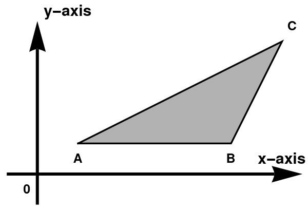
We demotstrate the validity of Green's formula \eqref{EqGreen.1} for triangular domain in the following example.
Example 2: ■
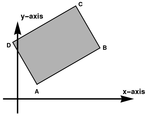
Finally, we consider arbitrarily oriented rectangular domain.
https://math.libretexts.org/Bookshelves/Calculus/Calculus_(OpenStax)/16%3A_Vector_Calculus/16.04%3A_Greens_Theorem
Example 4: ■
- Find the area of the region enclosed by the curve with parameterization r(t) = (sint cost, sint).
- Use Green’s theorem to calculate line integral \( \displaystyle \quad \oint_C \sin \left( x^2 \right) {\text d}x + \left( 3 x - y^3 \right) {\text d} y , \quad \) where C is a right triangle with vertices (−2, 2), (4, 2), and (4, 7) oriented counterclockwise.
- Anton, Howard (2005), Elementary Linear Algebra (Applications Version) (9th ed.), Wiley International
- Beezer, R., A First Course in Linear Algebra, 2015.
- Beezer, R., A Second Course in Linear Algebra, 2013.