Introduction to Linear Algebra
Complex Variables
- Introduction
- Linear systems
- Vectors
- Linear combinations
- Matrices
- Planes in ℝ³
- Reduced Row-Echelon Form
- Equation A x = b
- Sensitivity of solutions
- Linear independence
- Plane transformations
- Space transformations
- Linear transformations
- Affine maps
- Exercises
- Answers
Series and Limits
- Introduction
- Manipulation of matrices
- Partitioned matrices
- Block matrices Matrix operators
- Determinants
- Cofactors
- Cramer's rule
- Equivalent matrices
- Elimination: A = L U
- PLU factorization
- Reflection
- Givens rotation
- Special matrices
- Exercises
- Answers
Differentiation
- Introduction
- Motivation
- Vector spaces
- Bases
- Dimension
- Coordinate systems
- Linear transformations
- Change of basis
- Matrix transformations
- Compositions
- Isomorphisms
- Dual transformations
- Direct sums
- Quotient spaces
- Rank
- Solving A x = b
- Exercises
- Answers
Integration
- Introduction
- Riemann integral
- Area and integral
- Properties of integration
- Primitive functions
- Fundamental theorem of calculus
- Integration by parts
- Indefinite integrals
- Improper integrals
- Double integral
- Polar coordinates
Vector Calculus
- Introduction
- Vector fields
- Paths
- Line integrals
- Inner product
- Gram--Schmidt Process
- Orthogonal sets
- Self-adjoint Matrices
- Unitary matrices
- Projection operators
- QR-decomposition
- Least Square Approximation
- Quadratic forms
- Exercises
- Answers
Tensors
- Introduction
- LU-decomposition
- QR-decomposition
- Cholesky decomposition
- Schur decomposition
- Positive matrices
- Roots
- Polar factorization
- Spectral decomposition
- Singular values
- SVD <
- Pseudoinverse
- Exercises
- Answers
Calculus of Variations
- Introduction
- GPS problem
- Poisson equation
- Graph theory
- Error correcting codes
- Electric circuits
- Markov chains
- Cryptography
- Wave-length transfer matrix
- Computer graphics
- Linear Programming
- Hill's determinant
- Fibonacci matrices
- Discrete dynamic systems
- Discrete Fourier transform
- Fast Fourier transform
- Curve fitting
Classical mechanics
- Introduction
- Similar matrices
- Diagonalization
- Sylvester formula
- The Resolvent method
- Polynomial interpolation
- Positive matrices
- Roots <
- Pseudoinverse
- Exercises
- Answers
Quantum mechanics
- Introduction
- Circles along curves
- TNB frames
- Tensors
- Tensors in ℝ³
- Tensors & Mechanics
- Differential forms
- Calculus
- Vector Representations
- Matrix Representations
- Change of Basis
- Orthonormal Diagonalization
- Generalized Inverse
- Differential forms
Preliminaries
- Complex Number Operations
- Sets
- Polynomials
- Polynomials and Matrices
- Computer solves Systems of Linear Equations
- Location of Eigenvalues
- Power Method
- Iterative Method
- Similarity and Diagonalization
Glossary
Reference

This Book is licensed under Creative Commons Attribution-NonCommercial-NoDerivs 3.0 Unported License
Green's Theorems in Polar coordinate
Semi-infinite strip
Let U ⊂ ℝ² be an open set containing a compact, simply-connected region Ω whose boundary is parameterized by the piecewise smooth, simple closed curve C = ∂Ω. Take C to be positively oriented when region Ω is at its left. Given functions P and Q defined on U such that {P, Q} ∈ ℭ¹(U), we have the following identityLet us consider the infinite half-strip RT = {(x, y) ∈ ℝ² : 0 ≤ x < ∞, 0 ≤ y < T < ∞}. This semi-infinite strip is a limit of enclosed bounded rectangles RT, n = {(x, y) ∈ ℝ² : 0 ≤ x < n, 0 ≤ y < T < ∞} whose boundary is parameterized by γ₁, γ₂, γ₃, and γ₄.
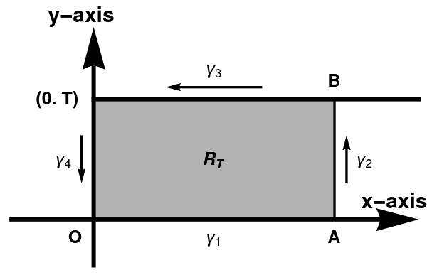
We would like to apply Green’s theorem to this region. However, since the theorem concerns a compact domain of integration, we must examine a sequence of closed and bounded sub-domains RT, n whose limit is RT.
The rectangle in the depiction Figure 1 above of RT, n has width 𝑎n, which is the nth term in the arbitrary positive sequence {𝑎n} → ∞ as n → ∞. Without any loss of generality, we can set 𝑎n = n.
If P and Q satisfy the conditions for Green’s theorem and if
- {P(x, 0), P(x, T)} are Lebesque integrable on half-line, which we abbreviate as ℌ¹(ℝ≥0);
- Q(𝑎n, y) → 0 pointwise on [0, T];
- Q(x, y) is uniformly bounded on y ∈ [0, T] for sufficiently large x;
- (Qx − Py) ∈ ℌ¹(ℝT);
I) By condition I and the continuity of the absolute value, \begin{align*} \left\vert \lim_{n\to\infty} \int_0^{a_n} P(x, 0)\,{\text d} x \right\vert &= \lim_{n\to\infty} \left\vert \int_0^{a_n} P(x, 0)\,{\text d} x \right\vert \\ &\le \lim_{n\to\infty} \int_0^{a_n} \left\vert P(x, 0) \right\vert {\text d} x = \int_0^{\infty} \left\vert P(x, 0) \right\vert {\text d} x < \infty . \end{align*} Similarly, \begin{align*} \left\vert \lim_{n\to\infty} \int_{a_n}^0 P(x, T)\,{\text d} x \right\vert &= \lim_{n\to\infty} \left\vert \int_0^{a_n} P(x, T)\,{\text d} x \right\vert \\ &\le \lim_{n\to\infty} \int_0^{a_n} \left\vert P(x, T) \right\vert {\text d} x = \int_0^{\infty} \left\vert P(x, T) \right\vert {\text d} x < \infty . \end{align*} We also know that \[ \left\vert \lim_{n\to\infty} \int_T^0 Q(0, y)\,{\text d}y \right\vert = \left\vert \int_0^T Q(0, y)\,{\text d}y \right\vert < \infty \] since Q is continuous on RT, n and the interval [0, T] is compact.
II, III) In order for \[ \lim_{n\to\infty} \int_0^T Q(a_n , y)\,{\text d}y = 0 \] we make use of conditions II and III. Let fn(y) := Q(𝑎n, y). Then for arbitrary fixed y ∈ [0, T], we have \( \displaystyle \quad \lim_{n\to\infty} f_n (y) = 0 . \)
According to condition III, there exists some N ∈ ℕ and a corresponding c₀ > 0 such that whenever n ≥ N, Q(𝑎n, y) ≤ c₀ for all y ∈ [0, T]. Define hn(y) := fN+n(y), and let g(y) := c₀ be a constant function. The function g dominates hn(y) on [0, T], as for all n ∈ ℕ, \[ \left\vert h_n (y) \right\vert = \left\vert f_{N+n} (y) \right\vert = \left\vert Q(a_{N+n} , y) \right\vert \le c_0 = g(y) . \] Moreover, g is integrable over the compact set [0, T], and hn is measurable. By the dominated convergence theorem \[ \lim_{n\to\infty} \int_0^T h_n (y)\,{\text d}y = \int_0^T \lim_{n\to\infty} h_n (y)\,{\text d}y = 0 . \] Notice that this result implies that \begin{align*} \lim_{n\to\infty} \int_0^T Q( a_n , y)\,{\text d}y &= \lim_{n\to\infty} \int_0^T f_n (y) \,{\text d}y = \lim_{n\to\infty} \int_0^T f_{N+n} (y) \,{\text d}y \\ &= \lim_{n\to\infty} \int_0^T h_n (y) \,{\text d}y = 0 . \tag{T1.1} \end{align*} We have proved the limit of each term in the sum converges and can reexpress the left-hand side of Green’s formula, \begin{align*} \mbox{LHS} &= \lim_{n\to\infty} \oint_{C_n} P\,{\text d}x + Q\,{\text d}y = \lim_{n\to\infty} \left( \int_0^{a_n} P(x,0)\,{\text d}x + \int_0^T Q( a_n , y)\,{\text d}y \right. \\ &\quad \left. + \int_{a_n} P(x, T)\,{\text d}x + \int_Y^0 Q(0, y) \,{\text d}y \right) \\ &= \lim_{n\to\infty} \int_0^{a_n} P(x,0)\,{\text d}x + \lim_{n\to\infty} \int_0^T Q( a_n , y)\,{\text d}y \\ &\quad + \lim_{n\to\infty} \int_{a_n} P(x, T)\,{\text d}x +\lim_{n\to\infty} \int_T^0 Q(0, y)\,{\text d}y \\ &= \int_0^{\infty} P(x,0)\,{\text d}x - \int_0^{\infty} P(x,T)\,{\text d}x - \int_0^{\infty} Q(0, y)\,{\text d}y . \end{align*}
IV) To deal with the limit of the sequence of area integrals in the right-hand side of Green’s formula, we first see that \[ \lim_{n\to\infty} \iint_{R_{T,n}} \left( Q_x - P_y \right) {\text d}A = \lim_{n\to\infty} \iint_{R_{T,n}} \mathbb{I}_{R_{T,n}} (x, y) \cdot \left( Q_x - P_y \right) {\text d}A . \] Next, define \( \displaystyle \quad f_N (x, y) = \mathbb{I}_{R_{T,n}} \cdot \left( \frac{\partial Q}{\partial x} - \frac{\partial P}{\partial y} \right) \quad \) for all (x, y) ∈ RT. Then \begin{align*} \lim_{n\to\infty} f_n (x,y) &= \lim_{n\to\infty} \left[ \mathbb{I}_{R_{T,n}} \cdot \left( Q_x - P_y \right) \right] \\ &= \lim_{n\to\infty} \mathbb{I}_{R_{T,n}} \cdot \left( Q_x - P_y \right) \\ &= \mathbb{I}_{R_T} (x, y) \cdot \cdot \left( Q_x - P_y \right) . \end{align*} We also know that \begin{align*} \left\vert f_n (x, y) \right\vert &= \left\vert \mathbb{I}_{R_T} (x, y) \cdot \cdot \left( Q_x - P_y \right) \right\vert = \mathbb{I}_{R_T} (x, y) \cdot \cdot \left\vert Q_x - P_y \right\vert \\ & \le \left\vert Q_x - P_y \right\vert \in ℌ¹(R_T) \end{align*} because of condition IV. Set g(x, y) = |Qx − Py| to be the dominating function for sequence fn.
Given that Qx − Py is measurable, and hence fn(x, y) is measurable, we can pass the limit into the integral using the dominated convergence theorem: \begin{align*} \lim_{n\to\infty} \iint_{R_{T,n}} \left( Q_x - P_y \right) {\text d}A &= \lim_{n\to\infty} \iint_{R_{T,n}} \mathbb{I}_{R_{T,n}} (x, y) \cdot \cdot \left( Q_x - P_y \right) {\text d}A \\ &= \lim_{n\to\infty} \iint_{R_T} f_n (x,y)\,{\text d}A \tag{????} \\ &= \iint_{R_T} \lim_{n\to\infty} \,f_n (x,y)\,{\text d}A = \iint_{R_T} \left( Q_x - P_y \right) {\text d}A . \end{align*} Therefore, if L and M satisfy the conditions set in Theorem 1, the left-hand side in Eq.(1) is \begin{align*} \mbox{LHS} &= \int_0^{\infty} P(x,0)\,{\text d}x - \int_0^{\infty} P(x,T)\,{\text d}x - \int_0^T Q(0, y)\,{\text d}y \\ &= \lim_{n\to\infty} \oint_{C_n} P(x, y)\,{\text d}x + Q(x,y)\,{\text d}y \\ &= \lim_{n\to\infty} \iint_{R_{T,n}} \left( Q_x - P_y \right) {\text d}A = \iint_{R_T} \left( Q_x - P_y \right) {\text d}A . \end{align*}
Application to the generalized heat equation
We would like to solve the following equation, which comes from analysis of the generalized heat equation,
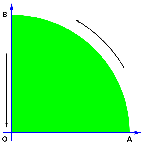
First quadrant in in Polar coordinates
A two-dimensional vector field F can be written in either Cartesian or polar coordinates: