
Introduction to Linear Algebra
Complex Variables
- Introduction
- Linear systems
- Vectors
- Linear combinations
- Matrices
- Planes in ℝ³
- Reduced Row-Echelon Form
- Equation A x = b
- Sensitivity of solutions
- Linear independence
- Plane transformations
- Space transformations
- Linear transformations
- Affine maps
- Exercises
- Answers
Series and Limits
- Introduction
- Definition of derivative
- Geometric meaning
- Properties Matrix operators
- Determinants
- Cofactors
- Cramer's rule
- Equivalent matrices
- Elimination: A = L U
- PLU factorization
- Reflection
- Givens rotation
- Special matrices
- Exercises
- Answers
Differentiation
- Introduction
- Definition of derivative
- Geometric meaning
- Properties Compositions
- Derivative of inverse
- Power rule
- Right and Left-hand derivatives
- Higher order derivatives
- Infinitesimals
- Differentials
- Extrema of a real-valued functions
- Fermat's and Rolle's theorems
- Lagrange theorem
- de l'Hospital's rule
- Dual transformations
- Direct sums
- Quotient spaces
- Rank
- Solving A x = b
- Exercises
- Answers
Integration
- Introduction
- Riemann integral
- Area and integral
- Properties of integration
- Primitive functions
- Fundamental theorem of calculus
- Integration by parts
- Indefinite integrals
- Improper integrals
- Lebesgue integral
- Properties
- Double integral
- Polar coordinates
- Self-adjoint operators
Vector Calculus
- Introduction
- Vector fields
- Paths
- Line integrals
- Inner product
- Norm and distance
- Matrix norms
- Dual norms
- Dual transformations
- Examples of transformations
- Exercises
- Answers
Tensors
- Introduction
- LU-decomposition
- QR-decomposition
- Cholesky decomposition
- Schur decomposition
- Positive matrices
- Roots
- Polar factorization
- Spectral decomposition
- Singular values
- SVD <
- Pseudoinverse
- Exercises
- Answers
Calculus of Variations
- Introduction
- GPS problem
- Poisson equation
- Graph theory
- Error correcting codes
- Electric circuits
- Markov chains
- Cryptography
- Wave-length transfer matrix
- Computer graphics
- Linear Programming
- Hill's determinant
- Fibonacci matrices
- Discrete dynamic systems
- Discrete Fourier transform
- Fast Fourier transform
- Curve fitting
Classical mechanics
- Introduction
- Similar matrices
- Diagonalization
- Sylvester formula
- The Resolvent method
- Polynomial interpolation
- Positive matrices
- Roots <
- Pseudoinverse
- Exercises
- Answers
Quantum mechanics
- Introduction
- Circles along curves
- TNB frames
- Tensors
- Tensors in ℝ³
- Tensors & Mechanics
- Differential forms
- Calculus
- Vector Representations
- Matrix Representations
- Change of Basis
- Orthonormal Diagonalization
- Generalized Inverse
- Differential forms
Preliminaries
- Complex Number Operations
- Sets
- Polynomials
- Polynomials and Matrices
- Computer solves Systems of Linear Equations
- Location of Eigenvalues
- Power Method
- Iterative Method
- Similarity and Diagonalization
Glossary
Reference

This Book is licensed under Creative Commons Attribution-NonCommercial-NoDerivs 3.0 Unported License
Green's Theorems in Polar coordinates
Besides rectangular coordinates, it is convenient to consider polar coordinates on ℝ². They originated in the work by the ancient Greek astronomer and astrologer Hipparchus (190–120 BC). The full history of the subject is described in Harvard professor Julian Lowell Coolidge's Origin of Polar Coordinates.In order to introduce polar coordinates, start with a point O in the plane ℝ² called the pole (we will always identify this point with the origin). From the pole, draw a ray, called the initial ray (we will always draw this ray horizontally, identifying it with the positive abscissa). A point P in the plane is determined by the distance r that P is from O, and the angle θ formed between the initial ray and the segment \( \displaystyle \quad \overline{OP} \quad \) (measured counter-clockwise). We record the distance and angle as an ordered pair (r, θ), which is known as polar notation. This representation is illustrated in the following figure:
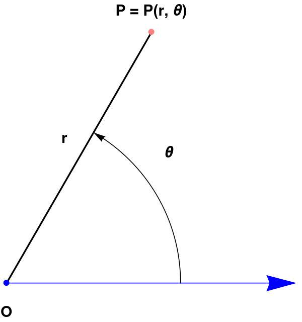
Conversion between rectangular and polar coordinates are based on the relations:
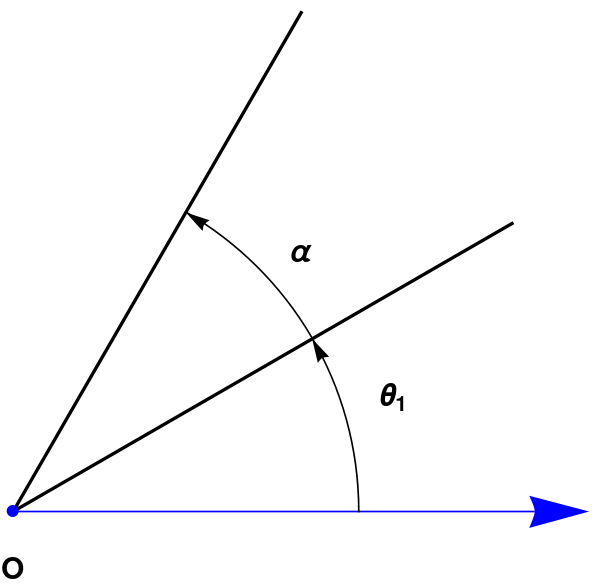
In order to preserve a unique representation of a point on the plane in polar coordinates as ordered pair (r, θ), the corresponding angle θ is taken within the interval of length 2π (if measured in radians) or 360 (if angle θ is measured in degrees). We assume that θ ∈ (−π, π] because we use radians; however, some authors prefer to use semi-open interval [0, 2π) or [0, 360°) in case of degrees. So the angle θ is defined according to the formula:
We summarize possible outputs in the following table.
| Quadrant | Range | Value |
| 1st (x > 0, y > 0) | 0 < θ < π/2 | θ = α |
| 2nd (x < 0, y > 0) | π/2 < θ < π | θ = π − α |
| 3rd (x < 0, y < 0) | −π < θ < −π/2 | θ = −π + α |
| 4th (x > 0, y < 0) | −π/2 < θ < 0 | θ = −α |
Defining a new coordinate system allows us to create a new kind of function, a polar function. Rectangular coordinates lent themselves well to creating functions that related x and y, such as y = sin(x). Polar coordinates allow us to create functions that relate r and θ. Normally these functions look like r = f(θ), although we can create functions of the form θ = g(r).
A polar curve can be parametrized by θ or by any parameter. The arc length of a polar curve given by r = r(θ) is
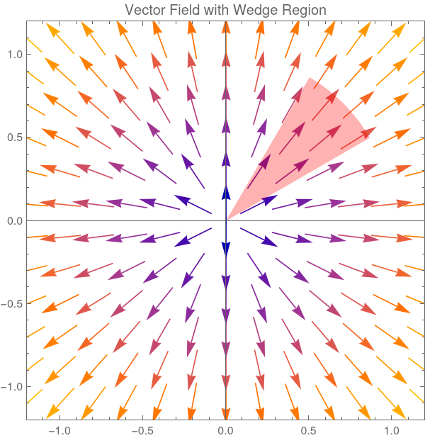
The basic rectangular equations of the form x = h and y = k create vertical and horizontal lines, respectively; the basic polar equations r = h and θ = α create circles and lines through the pole, respectively. A typical example of this form is a wedge:
We choose a finite part of the wedge bounded by 0 < r ≤ 𝑎 for some positive 𝑎:
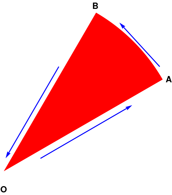
The boundary ∂Wedge of our domain consists of two lines, OA and BO, and a part of circle r = 𝑎 (θ₁ ≤ θ ≤ θ₂). We want to integrate an arbitrary vector field
Now we integrate over the arc of circle AB; note that dr = 0 on this piece because variable r is constant. So
Cos[\[Theta]] f\[Theta][r, \[Theta]] + fr[r, \[Theta]] Sin[\[Theta]]
Cos[\[Theta]] (Cos[\[Theta]] f\[Theta][r, \[Theta]] + fr[r, \[Theta]] Sin[\[Theta]]) - Sin[\[Theta]] (Cos[\[Theta]] fr[r, \[Theta]] - f\[Theta][r, \[Theta]] Sin[\[Theta]])
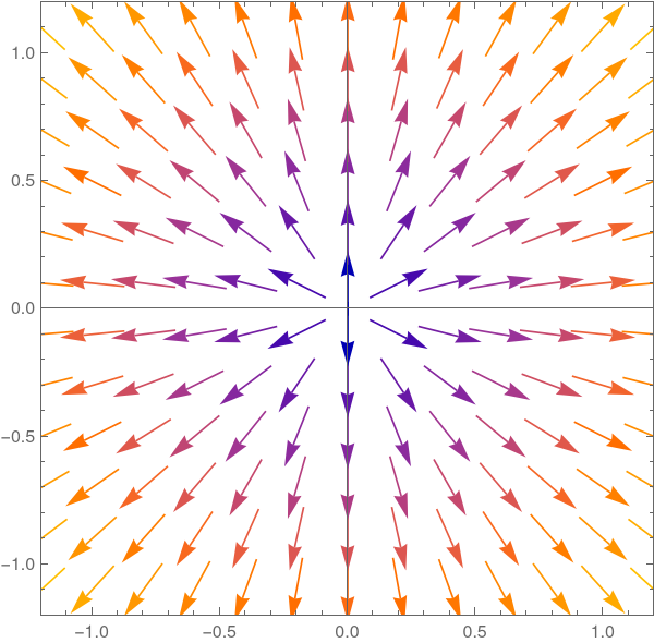
Here is code that implements the above manipulations to replicate the wedge graphic we started with and the vector field in which it lies. First we define specific functions for fr and fθ:
Before formulating Green's theorem, we remind some definitions. A rectifiable curve is a curve having finite length. If curve does not cross itself, it is called a simple curve.
Let F be a vector field on the plane: \[ \mathbf{F} = F_r \hat{\bf e}_r + F_{\theta}\hat{\bf e}_{\theta} , \] which we want to integrate around a closed path ∂R containing a simple domain R. First, we make connection polar coordinate representation with its Cartesian one: \begin{align*} \mathbf{F} &= P(x,y)\,{\bf i} + Q(x,y)\,{\bf j} = F_r \hat{\bf e}_r + F_{\theta}\hat{\bf e}_{\theta} \\ &= F_r \left( \cos\theta\,{\bf i} + \sin\theta\,{\bf j} \right) + F_{\theta} \left( -\sin\theta\,{\bf i} + \cos\theta\, {\bf j} \right) \\ &= \left( F_r \cos\theta - F_{\theta} \sin\theta \right) {\bf i} + \left( F_r \sin\theta + F_{\theta} \cos\theta \right) {\bf j} . \end{align*} We know that partial derivatives in rectangular coordinates are expressed through partial derivatives of polar coordinates as \[ \frac{\partial}{\partial x} = \cos\theta\,\frac{\partial}{\partial r} - \frac{\sin\theta}{r} \,\frac{\partial}{\partial \theta} , \qquad \frac{\partial}{\partial y} = \sin\theta\,\frac{\partial}{\partial r} + \frac{\cos\theta}{r} \,\frac{\partial}{\partial \theta} . \] Therefore, \begin{align*} \frac{\partial Q}{\partial x} &= \left( \cos\theta\,\frac{\partial}{\partial r} - \frac{\sin\theta}{r} \,\frac{\partial}{\partial \theta} \right) \left[ F_r \sin\theta + F_{\theta} \cos\theta \right] \\ &= \cos\theta \left( \frac{\partial F_r}{\partial r} \cdot \sin\theta + \frac{\partial F_{\theta}}{\partial r} \cdot \cos\theta\right) \\ & \quad - \frac{\sin\theta}{r} \left( \frac{\partial F_r}{\partial \theta} \cdot \sin\theta + F_r \cos\theta + \frac{\partial F_{\theta}}{\partial \theta} \cdot \cos\theta - F_{\theta} \sin\theta \right) \end{align*} Similarly, \begin{align*} - \frac{\partial P}{\partial y} &= - \left( \sin\theta\,\frac{\partial}{\partial r} + \frac{\cos\theta}{r}\,\sin\theta\,\frac{\partial}{\partial \theta} \right) \left[ F_r \cos\theta - F_{\theta} \sin\theta \right] \\ &= - \sin\theta \left( \frac{\partial F_r}{\partial r} \cdot \cos\theta - \frac{\partial F_{\theta}}{\partial r} \cdot \sin\theta \right) \\ & \quad - \frac{\cos\theta}{r} \left( \frac{\partial F_r}{\partial \theta} \cdot \cos\theta - F_r \sin\theta - \frac{\partial F_{\theta}}{\partial \theta} \cdot \sin\theta - F_{\theta} \cos\theta \right) . \end{align*} Summing up, \begin{align*} \frac{\partial Q}{\partial x} - \frac{\partial P}{\partial y} &= \frac{1}{r} \left( \frac{\partial}{\partial r} \left( r\,F_{\theta} \right) - \frac{\partial F_r}{\partial \theta} \right) = \mbox{curl}(\mathbf{F}) \bullet \mathbf{k} , \end{align*} where k = (0, 0, 1) is a unit vector along applicate axis (usually denoted by z).
We use Green's theorem.

 |
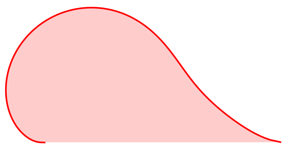 |
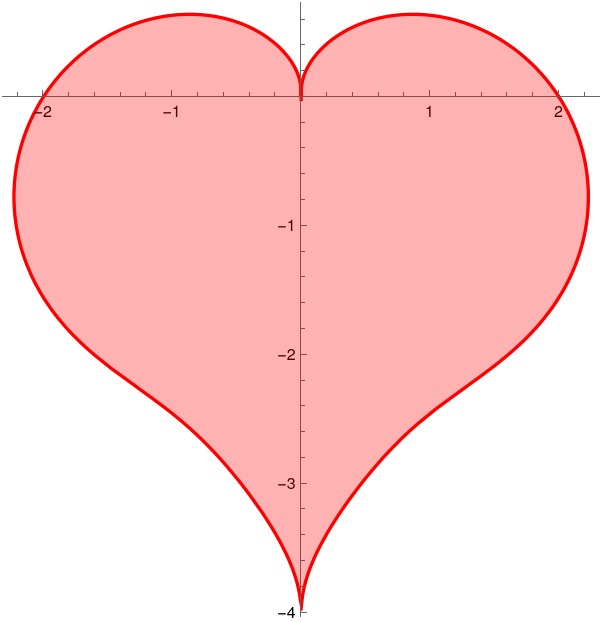
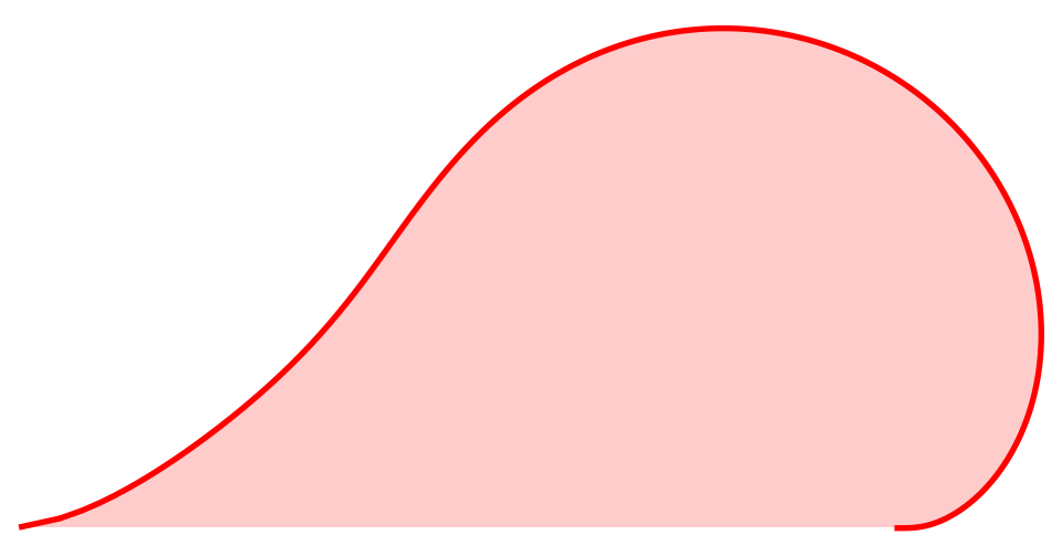
Define the parametric equations for the rotated heart - like curve
- Coolidge, J.L., The Origin of Polar Coordinates, American Mathematical Monthly. 1952, volume 59, issue 2, pp. 78–85. doi:10.2307/2307104.
- Fleming, W., Functions of Several Variables, Undergraduate Texts in Mathematics, Second edition, Springer-Verlag, New York–Heidelberg, 1977.
- Hubbard, J.H. and Hubbard, B.B., Vector Calculus, Linear Algebra, and Differential Forms: A Unified Approach, Matrix Editions; 5th edition, 2015; ISBN-13: 978-0971576681