Return to computing page for the first course APMA0330
Return to computing page for the second course APMA0340
Return to computing page for the fourth course APMA0360
Return to Mathematica tutorial for the first course APMA0330
Return to Mathematica tutorial for the second course APMA0340
Return to Mathematica tutorial for the fourth course APMA0360
Return to the main page for the course APMA0330
Return to the main page for the course APMA0340
Return to the main page for the course APMA0360
Introduction to Linear Algebra with Mathematica
Glossary
Preface
The following theorem is credited to a British mathematical physicist George Green (1793--1841), who stated a similar result in an 1828 paper titled An Essay on the Application of Mathematical Analysis to the Theories of Electricity and Magnetism. In 1846, the form of "Green's theorem" was first published, without proof, in an article by Augustin Cauchy (1789--1857): A. Cauchy (1846) "Sur les intégrales qui s'étendent à tous les points d'une courbe fermée" (On integrals that extend over all of the points of a closed curve), Comptes rendus, 23: 251–255. A proof of the theorem was finally provided in 1851 by Bernhard Riemann (1826--1866) in his inaugural dissertation: Bernhard Riemann (1851) Grundlagen für eine allgemeine Theorie der Functionen einer veränderlichen complexen Grösse (Basis for a general theory of functions of a variable complex quantity), (Göttingen, (Germany): Adalbert Rente, 1867)
Green's formular for rectangular domains
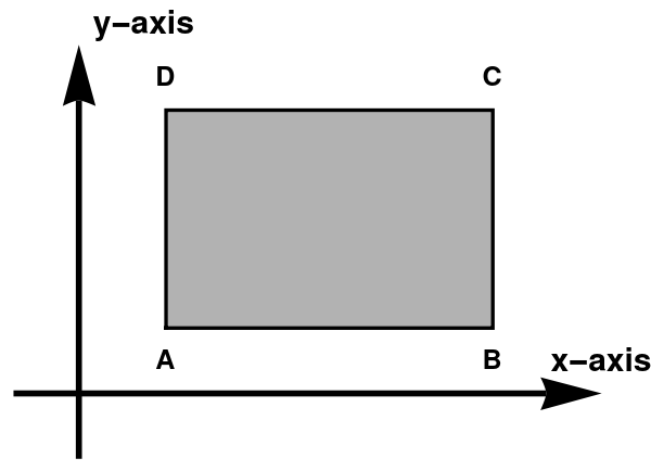
We consider a rectangle R in ℝ² oriented along Cartersian axes.
|
original = Polygon[{{0, 0}, {1.5, 0}, {1.5, 1}, {0, 1}}];
rec = Graphics[{EdgeForm[{Thick, Black}], Opacity[.3], Black,
original, LightRed}, Axes -> False]
arx = Graphics[{Black, Thickness[0.01], Arrowheads[0.1],
Arrow[{{-0.7, -0.3}, {2, -0.3}}]}]; ary =
Graphics[{Black, Thickness[0.01], Arrowheads[0.1],
Arrow[{{-0.4, -0.6}, {-0.4, 1.3}}]}];
txt = Graphics[{Black,
Text[Style["A", FontSize -> 15, Bold], {0, -0.15}],
Text[Style["x-axis", FontSize -> 18, Bold], {2.0, -0.15}],
Text[Style["B", FontSize -> 15, Bold], {1.5, -0.15}],
Text[Style["y-axis", FontSize -> 18, Bold], {-0.1, 1.4}],
Text[Style["C", FontSize -> 15, Bold], {1.5, 1.15}],
Text[Style["D", FontSize -> 15, Bold], {0, 1.15}]}];
Show[rec, arx, ary, txt]
|
| Figure 1: Rectangualr domain. | Mathematica code. |
Example 1: ■
|
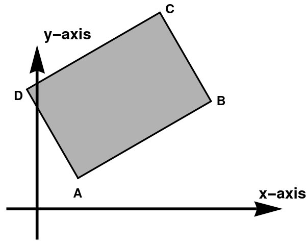
trans = Polygon[{{0, 0}, {1.5*Sqrt[3]/2, 1.5/2}, {0.799,
1.6160254037844}, {-1/2, Sqrt[3]/2}}]
recT = Graphics[{EdgeForm[{Thick, Black}], Opacity[.3], Black, trans,
Blue}, Axes -> False]
txt = Graphics[{Black,
Text[Style["A", FontSize -> 15, Bold], {0, -0.15}],
Text[Style["x-axis", FontSize -> 18, Bold], {2.0, -0.15}],
Text[Style["B", FontSize -> 15, Bold], {1.4, 0.75}],
Text[Style["y-axis", FontSize -> 18, Bold], {-0.1, 1.4}],
Text[Style["C", FontSize -> 15, Bold], {0.9, 1.65}],
Text[Style["D", FontSize -> 15, Bold], {-0.58, 0.8}]}];
Show[recT, arx, ary, txt]
|
| Figure 2: Rectangualr domain. | Mathematica code. |
Example 2: ■
Green's formular for a semi-infinite strip
Green's formular for general domains
In physical systems it is usual to define a scalar or vector field in some region R. In the next and some later sections we will need the concept of the connectivity of such a region in both two and three dimensions.
A plane region R is said to be simply connected if every simple closed curve within R can be continuously shrunk to a point without leaving the region (see figure). If, however, the region R contains a hole then there exist simple closed curves that cannot by shrunk to a point without leaving R (see figure 11.2(b)). Such a region is said to be doubly connected, since its boundary has two distinct parts. Similarly, a region with n − 1 holes is said to be n-fold connected, or multiply connected (the region in figure 11.2(c) is triply connected).
We consider line integrals for which the path C is closed and lies entirely in the xy-plane. Since the path is closed it will enclose a region R of the plane. We now discuss how to express the line integral around the loop as a double integral over the enclosed region R.
Suppose the functions P(x, y), Q(x, y) and their partial derivatives are single-valued, finite and continuous inside and on the boundary C = &partial;R of some simply connected region R in the xy-plane. Green’s theorem in a plane then states
- Apostol, Tom (1960). Mathematical Analysis. Reading, Massachusetts, U.S.A.: Addison-Wesley.
Return to Mathematica page
Return to the main page (APMA0340)
Return to the Part 1 Basic Concepts
Return to the Part 2 Fourier Series
Return to the Part 3 Integral Transformations
Return to the Part 4 Parabolic PDEs
Return to the Part 5 Hyperbolic PDEs
Return to the Part 6 Elliptic PDEs
Return to the Part 6P Potential Theory
Return to the Part 7 Numerical Methods