

Bernoulli Equations
A differential equation
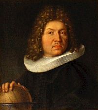
Bernoulli returned to Switzerland and began teaching mechanics at the University in Basel from 1683. In 1684 he married Judith Stupanus. They had two children. He was appointed professor of mathematics at the University of Basel in 1687, remaining in this position for the rest of his life. By that time, he had begun tutoring his younger brother Johann Bernoulli on mathematical topics. The two brothers began to study the calculus as presented by Leibniz in his 1684 paper on the differential calculus. Jacob collaborated with his brother on various applications of calculus. However the atmosphere of collaboration between the two brothers turned into rivalry as Johann's own mathematical genius began to mature, with both of them attacking each other in print, and posing difficult mathematical challenges to test each other's skills. By 1697, the relationship had completely broken down.
Jacob Bernoulli is known for his numerous contributions to calculus, and along with his brother Johann, was one of the founders of the calculus of variations. In May 1690, in a paper published in Acta Eruditorum, Jacob Bernoulli showed that the problem of determining the isochrone is equivalent to solving a first-order nonlinear differential equation. The isochrone, or curve of constant descent, is the curve along which a particle will descend under gravity from any point to the bottom in exactly the same time, no matter what the starting point. He also discovered the fundamental mathematical constant e, which Euler later denoted by e.
Jacob made a great contribution to calculus. By 1689 he had published important work on infinite series and showed that harmonic series diverges, which had actually been proved by Mengoli 40 years earlier. Jacob Bernoulli also discovered a general method to determine evolutes of a curve as the envelope of its circles of curvature. He also investigated caustic curves and in particular he studied these associated curves of the parabola, the logarithmic spiral and epicycloids around 1692. The lemniscate of Bernoulli was first conceived by Jacob Bernoulli in 1694. In 1695 he investigated the drawbridge problem which seeks the curve required so that a weight sliding along the cable always keeps the drawbridge balanced.
However, his most important contribution was in the field of probability, where he derived the first version of the law of large numbers in his work Ars Conjectandi, published in Basel in 1713, eight years after his death.Jacob Bernoulli chose a figure of a logarithmic spiral (its equation in polar coordinates is \( r = a\, e^{b\,\theta} \) ) and the motto Eadem mutata resurgo ("Changed and yet the same, I rise again") for his gravestone; the spiral executed by the stonemasons was, however, an Archimedean spiral, \( r = a + b\, \theta . \)
Bernoulli equations are special because they are nonlinear differential equations with known exact solutions. Moreover, they do not have singular solutions---similar to linear equations. There are two methods known to determine its solutions: one was discovered by Bernoulli himself, and another is credited to Gottfried Leibniz (1646--1716).
Leibniz substitution
The Bernoulli equation \( \quad y' + p(x)\,y = g(x)\,y^\alpha \quad \) can be reduced to a linear differential equation with substitution
This method is implemented in Maple:
ode;
y[t_] = x[t]^(1 - n);
L[x_] := D[x, t] + p*x - q*x^n;
xSub[t_] = y[t]^(1/(1 - n));
a2 = Simplify[L[xSub[t]]];
a3 = a2/y[t]^(n/(1 - n));
Simplify[PowerExpand[a3]]
Bernoulli Method
ode;
ode;
solution = DSolve[y'[x] + 2 x y[x] == x^2 y[x]^3, y[x], x]
ode;
Example 1: Consider the differential equation \( \quad y\, y' = y^2 + e^x . \ \) Since in the given differential equation the derivative is not isolated, we divide both sides by y. As a result, we obtain a Bernoulli equation y′ = y + ex/y (here prime indicates differentiation: y′ = dy/dx). To solve it, we first use the Leibniz substitution: u = y². \( \displaystyle \quad \Longleftrightarrow \quad y = u^{1/2} . \quad \) Then \[ y' = \frac{1}{2}\, u^{-1/2} u' \quad \Longrightarrow \quad y\,y' = \frac{1}{2}\, u' \] and we get the linear differential equation with respect to unknown function u:
Now we demonstrate the application of the Bernoulli method by seeking the solution as the product y = u v, where u is a solution of the "linear part:"
Table[{Sqrt[-2 E^x + c E^(2 x)], -Sqrt[-2 E^x + c E^(2 x)]}, {c,
1/4, 3, 3/4}]] (* increment is 3/4 *) ;
{Sqrt[-2 E^x + E^(2 x)/4], -Sqrt[-2 E^x + E^(2 x)/4], Sqrt[-2 E^x +
E^(2 x)], -Sqrt[-2 E^x + E^(2 x)], Sqrt[-2 E^x + (7 E^(2 x))/
4], -Sqrt[-2 E^x + (7 E^(2 x))/4], Sqrt[-2 E^x + (5 E^(2 x))/
2], -Sqrt[-2 E^x + (5 E^(2 x))/2]} ;
Plot[Evaluate[curves], {x, 0, 4}, PlotRange -> All]

ode;
Example 2: The four streamlines
(corresponding to the values of an arbitrary constant C=1,2,3,4) from the
general solution y=1/(x Sqrt[C-2 ln[x]]) of the Bernoulli equation
x y' =x^2 y^3 -y can be plotted with one command:
ode;
ode;

|

|
|
| Some trajectories. | Direction field. |
■
Example 3:: Consider the Bernoulli equation \( y' +x\,y=x\, y^4 . \) Using Leibniz substitution
ode;
ode;
ode;
ode;
Now we find the general solution using the Bernoulli method: y = u·v, where u is a solution of the "truncated" linear equation \( u' + x\,u =0 \) and v is the general solution of the separable equation \( u\, v' = x\, \left( u\, v \right)^4 . \) Solving the equation for u, we get
ode;
Example 4: (Logistic equation)
The logistic equation with harvesting \( \dot{y} = r\, y \left( 1 - \frac{y}{k} \right) - h\, y(t) \) is an example of the Bernoulli equation. It is assumed that all coefficients (r, k, h) are constants. It can be solved and plotted as follows.
DSolve[LogisticEquation, y, t]
{{y -> Function[{t}, -((E^(r t + h k C[1]) k (-h + r))/(
E^(h t + k r C[1]) - E^(r t + h k C[1]) r))]}}
ode;
{{y -> Function[{t}, (5 a E^(t/4))/(5 - a + a E^(t/4))]}}
ode;
To plot the results, we employ two options:
{-((25 E^(t/4))/(10 - 5 E^(t/4))), -((20 E^(t/4))/(
9 - 4 E^(t/4))), -((15 E^(t/4))/(8 - 3 E^(t/4))), -((10 E^(t/4))/(
7 - 2 E^(t/4))), -((5 E^(t/4))/(6 - E^(t/4))), 0, (5 E^(t/4))/(
4 + E^(t/4)), (10 E^(t/4))/(3 + 2 E^(t/4)), (15 E^(t/4))/(
2 + 3 E^(t/4)), (20 E^(t/4))/(1 + 4 E^(t/4)), 5}
ode;

y[t] /. sol /. {{a -> 1}, {a -> -1}, {a -> -1.5}, {a -> 1.5}}], {t, -1, 5}, PlotRange -> All]
ode;

Solution: The slope of the tangent line to the curve is its derivative, y′(x) at any point x. First, we plot the picture. Setting some parameters,
k := 3:
a := 1:
y := x-> 2*exp(x/(2*a))*sqrt(a*(a+x)*exp(-x/a)- a^2 + k^2/4):
the_parabola := a*x:
xA := 1:
yA := y(xA):
yPrime:= x-> diff(y(x), x):
kSlope := -1/eval(yPrime(x),x=xA):
bIntercept := yA - kSlope*xA:
xB := -bIntercept/kSlope:
yB := 0:
xC := (xA + xB)/2:
yC := yA/2:

while abs(yC^2 - eval(the_parabola,x=xC)) > 1/1000 do
   xC := xC + 1/100;
   yC := sqrt(eval(the_parabola,x=xC));
od:

p1:=plottools:-line([xA,yA],[xB,yB],color="Blue"):
p2:=plot([y(x), sqrt(the_parabola)],x=-5..11, y=0..6):
plots:-display([p1,p2]);
the_parabola := a*x:
Choose a point A on the curve y = y(x)
xA := 1:
yA := y(xA):
Calculate the derivative of y(x)
yPrime:= x-> diff(y(x), x):
kSlope;
evalf(%);
kSlope;
evalf(%);
ode;
ode;
is( Student[Precalculus]:-Distance([xA, yA], [xC, yC]) = Student[Precalculus]:-Distance([xB, yB], [xC, yC]));
ode;

Is C at the midpoint of the line?
ode;
ode;
ode;
ode;
The slope of the normal line is k = −1/y′(x). With this in hand, we find the equation of the normal line y = k x + b that goes through an arbitrary point A(x, y) on the curve and crosses abscissa at B(X, 0). Since X belongs to the normal line, we obtain \[ 0 = k\,X + b \qquad \Longrightarrow \qquad X = - \frac{b}{k} = b\,y' (x) . \] Substituting y − k x instead of b, yields \[ X = - \frac{y-k\,x}{k} = x - \frac{y}{k} = x + y \cdot y' \] because k = −1/y′. The middle point C of the segment A B has coordinates (X₁, Y₁) that are mean values of corresponding coordinates A(x, y) and B(x + y·y′, 0), that is, \[ X_1 = \frac{x + x + y\,y'}{2} = x + \frac{y}{2} \, y' \quad\mbox{and} \quad Y_1 = \frac{y}{2} . \] The coordinates of point C satisfy the equation of the parabola, y² = 𝑎x. Thus, \[ Y_1^2 = \left( \frac{y}{2} \right)^2 = a\, X_1 \qquad \Longrightarrow \qquad X_1 = x + \frac{y}{2} \, y' = \frac{1}{a} \left( \frac{y}{2} \right)^2 \] or \[ \frac{{\text d} y}{{\text d}x} = \frac{y}{2a} - \frac{2x}{y} \tag{5.1} \] This is a Bernoulli equation. We plot the corresponding direction field and some typical solutions to Eq.(5.1).
NDSolve[{y'[x] == y[x]/2 - 2*x/y[x], y[0] == 3}, y, {x, 0, 2}];
sol3 = Plot[Evaluate[y[x] /. %], {x, 0, 2}, PlotStyle -> {Black, Thick}];
NDSolve[{y'[x] == y[x]/2 - 2*x/y[x], y[0] == 2}, y, {x, 0, 2}]; sol2 = Plot[Evaluate[y[x] /. %], {x, 0, 2}, PlotStyle -> {Black, Thick}];
NDSolve[{y'[x] == y[x]/2 - 2*x/y[x], y[0] == -3}, y, {x, 0, 2}]; sol3m = Plot[Evaluate[y[x] /. %], {x, 0, 2}, PlotStyle -> {Red, Thick}];
NDSolve[{y'[x] == y[x]/2 - 2*x/y[x], y[0] == -2}, y, {x, 0, 2}]; sol2m = Plot[Evaluate[y[x] /. %], {x, 0, 2}, PlotStyle -> {Red, Thick}];
Show[field, sol2, sol3, sol3m, sol2m]
ode;

ode;
DSolve[v'[x] == -2*x/(v[x]*u[x]*u[x]), v[x], x]
ode;
ode;
ode;

The following animation shows the function v(x) depending on the value of K.
ode;

Multiplying expression (5.4) by u(x), we get the explicit formulas for two branches of the solution: \[ y(x) = \pm 2\, e^{x/(2a)} \, \sqrt{a \left( a+x \right) e^{-x/a} - a^2 + K^2 /4} = \pm 2\, \sqrt{a \left( a+x \right) - a^2 e^{x/a} + e^{x/a} \,K^2 /4} . \tag{5.4} \] We check with Mathematica:
ode;
ode;
Now capabilities of a computer algebra systems (such as Mathematica) are so powerful that we can check equivalence of many transcendent expressions with one line command. Previously, people verified equivalence of two expressions (one is obtained using standard command DSolve and another one was derived manually based on the Bernoulli method) were forced to evaluate these expressions at some numerical values of parameters. For example, if we were 20 years ago, we would check these two answers numerically upon evaluating the corresponding expressions at some points; for instance, we evaluate at x = 1.55.
ode;
ode;
We plot both branches of the solution for two particular values of parameters: 𝑎 = 1 and K = 3.
ode;

- Find the general solution of the logistic equation: y′ = y(2 - 5y).
- Find a particular solution to the initial value problem: y′ = y²ex − y, y(0) = 1.
- Find the general solution of the Bernoulli equation: y′ = xy³ − 3y.
- Find a particular solution to the initial value problem: y′ = y²e3x + 4y, y(0) = −1.
- Find the general solution of the Bernoulli equation: y′ + 2 y + 4 xy³ = 0.
- For the Bernoulli equation y′ = y³ex − 2y, find the positive solution that separates solutions tending to zero from those having a vertical asymptote at a positive value of x. What is the initial value y(0) for this solution?
- Abbasi, N.M., Differential Equations Algorithms, 2024.
- Azevedo, D. and Valentino, M.C., Generalization of the Bernoulli ODE, International Journal of Mathematical Education in Science and Technology, 2017, Volume 48, Issue 2, pp. 256--260; doi:https://doi.org/10.1080/0020739X.2016.1201599
- Tisdell, C.C., Alternate solution to generalized Bernoulli equations via an integrating factor: an exact differential equation approach, International Journal of Mathematical Education in Science and Technology, 2017, Volume 48, Issue 6, pp. 913--918; doi: https://doi.org/10.1080/0020739X.2016.1272143