First Order Ordinary Differential Equations
This tutorial contains many Mathematica scripts. You, as the user, are free to use all codes for your needs, and have the
right to distribute this tutorial and refer to this tutorial as long as
this tutorial is accredited appropriately. I would like to extend my gratitude to all of the students that aided me in
developing this tutorial. The coding, testing, and debugging required a concerted effort, and the
following students deserve recognition for their input: Emmet and Jesse Golden-Marx (Fall 2011), Pawel Golyski (Fall 2012). Any comments and/or contributions for this tutorial are welcome; you can send your remarks to <Vladimir_Dobrushkin@brown.edu>
Return to
computing page
Return to
computing page for the second course APMA0330
Return to
Mathematica tutorial page for the first course
Return to
Mathematica tutorial page for the second course
Return to the
main page for the course APMA0330
Return to the
main page for the course APMA0340
Contents
Part II. First Order ODEs
Solving ODEs
Direction fields
Separable equations
Equations reducible to separable equations.
Exact equations
Integrating Factors
Linear and Bernoulli equations
Riccati equation
Existence and Uniqueness
Qualitative analysis
Applications
The Wolfram Language function
DSolve finds symbolic solutions to
differential equations. (The Wolfram Language function
NDSolve, on the
other hand, is a general numerical differential equation solver.)
DSolve can handle the following types of equations:
Ordinary Differential Equations (ODEs), in which there are two or more
independent variables and one dependent variable. Finding exact
symbolic solutions of ODEs is a difficult problem, but DSolve can
solve most first-order ODEs and a limited number of the second-order
ODEs found in standard reference books.
Partial Differential Equations (PDEs), in which there are two or more independent variables and one dependent variable. Finding exact symbolic solutions of PDEs is a difficult problem, but DSolve can solve most first-order PDEs and a limited number of the second-order PDEs found in standard reference books.
Differential_Algebraic Equations (DAEs), in which some members of the system are differential equations and the others are purely algebraic, having no derivatives in them. As with PDEs, it is difficult to find exact solutions to DAEs, but DSolve can solve many examples of such systems that occur in applications.
http://reference.wolfram.com/language/tutorial/DSolveIntroduction.html
I. Verification
Mathematica can also be used to verify that known functions are solutions to different differential equations. To verify that the function y=e^(2*x) is a solution of the differential equation y' - 2 y=0 type:
Clear[y,x]
y[x_]=Exp[2 x]
y'[x]-2 y[x]=0
If you enter this syntax correctly, you should get two outputs. The first output should read e^(2*x). You should get the second output by plugging this potential solution into the differential equation on the third line, which gives a result of zero.
Another example:
y[x_]=c Exp[x*x]
Simplify[y'[x]-2 x y[x] ==0]
In this syntax, Exp[ ] is the exponential command. It is necessary to make sure that you use the correct brackets. If you do not use the correct type of brackets then the command will not work. We also define a function of a given variable by placing that variable in brackets next to the function. To take derivatives you use '. This means "y-prime" in this context. When you enter this syntax, you once again get two outputs. The first
outputs tells you what the function you are defining as y[x_] is. The second output tells you that this statement is true and cannot be simplified.
Example 1.1.1:
Clear[y]
y[t_]=c1 Cos[a*t]+c2*Sin[a*t]
Simplify[y''[t]+a^2*y[t]==0]
In this syntax, you define Cosine and Sine by Cos[ ] and Sin[ ].
When you enter this syntax. You get a similar result to the previous trials. The first output tells you the equation that you defined. The second output tells you that the equation you are trying to simplify is true and cannot be simplified.
To verify that the function y=e^(2*x) is a solution of the differential equation y' - 2 y=0 type:
Clear[y,x]
y[x_]=Exp[2 x]
Out[2]= E^(2 x)
y'[x]-2 y[x]=0
Out[3]= 0
Another example:
y[x_]=c Exp[x*x]
Out[4]= c E^x^2
Simplify[y'[x]-2 x y[x] ==0]
Out[5]= True
Example 1.1.2:
Clear[y]
y[t_]=c1 Cos[a*t]+c2*Sin[a*t]
Out[7]= c1 Cos[a t] + c2 Sin[a t]
Simplify[y''[t]+a^2*y[t]==0]
Out[8]= True
Sometimes it is convenient to interchange dependent and independent variables.
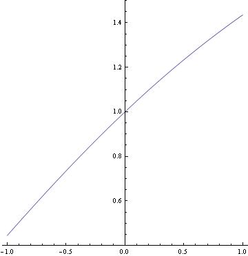
Example 1.1.3: First, we solve and plot the solution
ans1 = DSolve[{y'[x] == 1/(2*x - 3*y[x] + 5), y[0] == 1}, y[x], x]
Out[1]= {{y[x] -> 1/6 (7 + 4 x - 3 ProductLog[1/3 E^(1/3 + (4x)/3)])}}
Plot[y[x] /. ans1, {x, -1, 1}, PlotRange -> {0.4, 1.5}, AspectRatio -> 1]
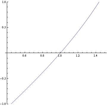
Here is the solution to the inverse problem:
ans2 = DSolve[{x'[y] == 2*x[y] - 3*y + 5, x[1] == 0}, x[y], y] // Simplify
Out[3]= {{x[y] -> 1/4 (-7 + E^(-2 + 2 y) + 6 y)}}
Plot[x[y] /. ans2, {y, 0.4, 1.5}, PlotRange -> {-1, 1}, AspectRatio -> 1]
Here is a way to flip the above graph:
ParametricPlot[Evaluate[{x[y], y} /. ans2], {y, 0, 2}, PlotRange -> {{-1, 1}, {0.4, 1.5}}, AspectRatio -> 1]
II. Plotting
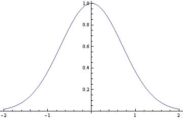
When Mathematica is capable to find a solution to the initial value problem, it can be plotted as follows
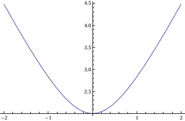
a = DSolve[{y'[x] == -2 x y[x], y[0] ==1}, y[x],x];
Plot[y[x] /.a, {x,-2,2}]
In this command sequence, I am first defining the differential equation that I want to solve. In this line, I define the equation and the initial condition as well as the independent and dependent variables.
In the second line, I am commanding Mathematica to evaluate the given differential equation and plot its result. I then command Mathematica to solve the equation and plot the given result of the initial value problem for the range listed above. Typing these two commands together allows Mathematica to solve the initial value problem for you and to graph the initial value problem's solution.
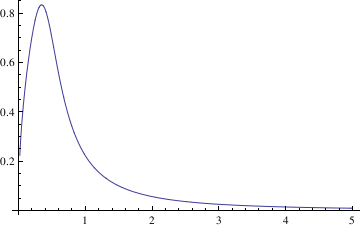
If you need to plot a sequence of solutions with different initial conditions, one can use the following script:
myODE = t^2*y'[t] == (y[t])^3 - 2*t*y[t]
IC = {{0.5, 0.7}, {0.5, 4}, {0.5, 1}};
Do[ansODE[i] =
Flatten[DSolve[{myODE, y[IC[[i, 1]]] == IC[[i, 2]]}, y[t], t]];
myplot[i] = Plot[Evaluate[y[t] /. ansODE[i]], {t, 0.02, 5}];
Print[myplot[i]]; , {i, 1, Length[IC]}]
Out[1]= t^2 Derivative[1][y][t] == -2 t y[t] + y[t]^3
DSolve::bvnul: For some branches of the general solution, the given
boundary conditions lead to an empty solution. >>
DSolve::bvnul: For some branches of the general solution, the given
boundary conditions lead to an empty solution. >>

DSolve::bvnul: For some branches of the general solution, the given
boundary conditions lead to an empty solution. >>
General::stop: Further output of DSolve::bvnul will be suppressed
during this calculation. >>
In this command, you define the differential equation that you want to solve and the initial conditions (the respective x and y values). Flattening creates a list of the equations. Then you are asking Mathematica to evaluate the different equations according to their different initial conditions.
Finally, the Print Command tells Mathematica to plot the graphs and the size that you want the lines on the graphs to be.
When you enter these commands, you may receive a line saying that some of the branches lead to empty solutions, but this just means that DSolve cannot find a unique solution for part of the equation. However, this does not appear to affect the final graph.
To plot a family of solutions:
f1[x_] = x*c + c/Sqrt[c*c + 1]
samples1 = Table[f1[x], {c, -20/3, 8, 1}]
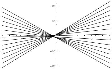
Plot[Evaluate[samples1], {x, -3, 3}, PlotStyle -> {Black}]
In this command, I am plotting a family of solutions to a differential equation. This command is not really any different from a normal plot command. The primary difference is that I have created a list of samples in a table. These samples have the variable c and then I can plug in different values of c to create the values in this table. This means that I am asking Mathematica to plot solutions with different values of the differential constant c. This command will plot a variety of different graphs over the range of c. The command on the second line also yields the different members of this family of equations associated with each value of c.
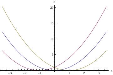
I can further complicate this problem by plotting a family of solutions to a differential equation along with the singular solution of the Initial Value Problem y' = 2sqrt(y), y(0)=0. To do this, use the following Mathematica code.
q1 = Plot[Evaluate[(x + C[1])^2 /. C[1] -> {0, 1, -1}], {x, -3.5, 3.5}, AxesLabel -> {x, y}]
q2 = Plot[y = x^2, {x, -3.5, 3.5}, PlotStyle -> Thick]
Show[q2, q1]
In this sequence of command, I am first entering the family of differential equations. Since I entered three values of C[1] I will get three graphs, each will be a different color. Then the second command will graph the solution to the initial value problem. By making this line thick, it will be easier for me to distinguish it. The final command graphs all of these curves on one graph.
Example. Plot tractrix curve, use the following code:
tractrix[a_][t_] := a*{Sin[t], Cos[t] + Log[Tan[t/2]]};
Manipulate[
ParametricPlot[tractrix[a][t] // Evaluate, {t, 0, .99*\[Pi]},
PlotRange -> {0, 7}], {a, 1, 6}]
Manipulate[
Plot[y'[x] = -Sqrt[a^2 - x^2]/x, {x, 0, 20},
PlotRange -> {-10, 10}], {a, 0, 20}]
sol = DSolve[{y'[x] == -Sqrt[a^2 - x^2]/x, y[a] == 0}, y, x]
Manipulate[
Plot[-Sqrt[a^2 - x^2] + a Log[a] - a Log[a^2] - a Log[x] +
a Log[a^2 + a Sqrt[a^2 - x^2]], {x, 0, 20}, PlotRange -> All], {a,
1, 20}]
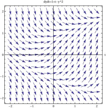
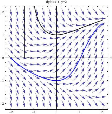
It is also very useful to use Mathematica to graph slope fields, or direction fields. A slope field is a graph that shows the value of a differential equation at any point in a given range. These are very tiresome to do by hand, so learning how to do this with a computer algebra system is incredibly useful. In Mathematica, the only one command is needed to draw the direction field corresponding to the equation y' =1+t-y^2:
dfield = VectorPlot[{1,1+t-y^2}, {t, -2, 2}, {y, -2, 2}, Axes -> True,
VectorScale -> {Small,Automatic,None}, AxesLabel -> {"t", "dydt=1+t-y^2"}]
In this command sequence the first thing that I do is define my equation as dfield.
After this, I entered the VectorPlot command. The first equation gives me the value of {dx,dy} because the slope field graphs dy/dx or dt in this example.
Then I defined the ranges for x and t for my graphs.
By commanding the Axes-> True, I am telling Mathematica to put all of the axes on the graph.
The option VectorScale allows one to fix the size of the arrows and Normalize makes the size of the arrows be 1.
The AxesLabel command just labels the two axes on this graph.
Another thing that is very useful to do is to plot the solution to one or more initial value problems on top of the direction field.
To plot the direction field along with, for example, two solutions, we
use the following commands:
sol1 = DSolve[{y'[t] == 1 - (y[t])^2 + t, y[0] == 1}, y[t], t]
sol2 = DSolve[{y'[t] == 1 - (y[t])^2 + t, y[0] == -1}, y[t], t]
pp1 = Plot[y[t] /. sol1, {t, -2, 2}]
pp2 = Plot[y[t] /. sol2, {t, -2, 2}]
Show[dfield, pp1, pp2]
In this command sequence, one first uses DSolve to solve the initial value differential equations. The third and fourth lines tells Mathematica to graph the two solutions to the initial value problem over a set range. The last command, show, tells Mathematica to show both the previously defined direction field, from the last example, and the two solutions to the differential equation. Since I just used an equal sign, =, when this command is entered I will see the solutions to the differential equations on separate graphs and then see a graph that has all three of these components on top of one another.
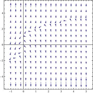
One can draw the direction field either with arrows
VectorPlot[{1, y^3 - 8*x}, {x, -1, 5}, {y, -5, 5}, VectorPoints -> 16, VectorStyle -> Arrowheads[0.028], Axes -> True]
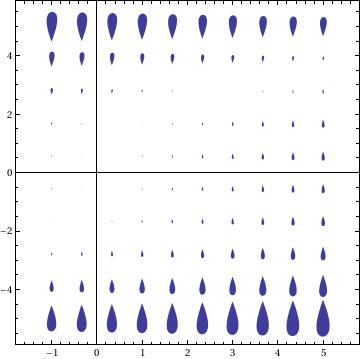
or with drop feature
VectorPlot[{1, y^3 - 8*x}, {x, -1, 5}, {y, -5, 5}, VectorPoints -> 10, VectorStyle -> "Drop", Axes -> True]
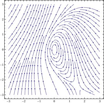
For plotting streamlines and their solutions, Mathematica has a dedicated command: StreamPlot. Streamlines are similar to vector lines except this command creates lines connecting the different values instead of arrows at each point.
The commands for this function are:
StreamPlot[{x^2 + y, y^2 - 4 x}, {x, -3, 3}, {y, -3, 3}]
This is a simple command. To use StreamPlot you use almost identical syntax to VectorPlot. The only difference is that for every command in which you use "Vector," you replace this with "Stream." You can also change the aesthetics of the graph in the same manner as VectorPlot.
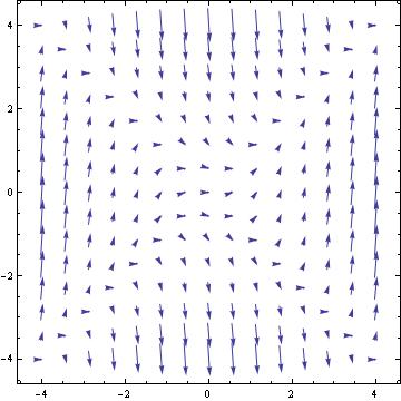
f[x_, y_] := x^2 - y^2
field = VectorPlot[{1, f[x, y]}, {x, -4, 4}, {y, -4, 4}, VectorStyle -> Arrowheads[0.025]]
Clear[y]
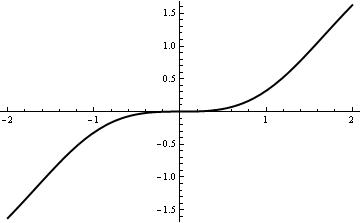
NDSolve[{y'[x] == f[x, y[x]], y[0] == 0}, y, {x, -2, 2}]
graph = Plot[Evaluate[y[x] /. %], {x, -2, 2}, PlotStyle -> {Black, Thick}]
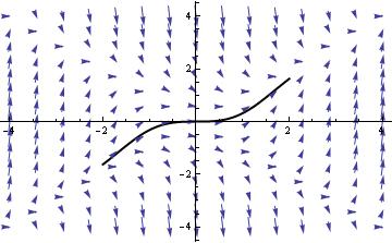
Show[graph, field, PlotRange -> Automatic]
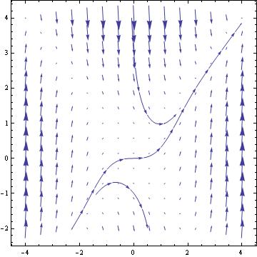
VectorPlot[{1, f[x, y]}, {x, -4, 4}, {y, -2, 4}, StreamPoints -> {{0, 0}, {0, -1}, {0, 3}}]
EqnA = DSolve[{y'[x]==x^2 -(y[x])^2, y[0]==0},y[x],x]
EqnB = DSolve[{y'[x]==x^2 -(y[x])^2, y[0]==-2},y[x],x]
EqnC = DSolve[{y'[x]==x^2 -(y[x])^2, y[0]==2},y[x],x]
Plot[{Evaluate[y[x]/.EqnA] , Evaluate[y[x]/.EqnB] ,Evaluate[y[x]/.EqnC]},
{x,-2,2},PlotStyle->Thickness[0.007]]
VectorPlot[{1, x^2 -y^2 },{x,-2,2},{y,-2,3},AxesLabel->{x,y[x]},
Axes->True, VectorPoints->15, VectorScale->{Tiny,Automatic,None},
StreamPoints ->8, StreamStyle->{Black,"Line"}]
sol = DSolve[{y'[x] == x^2 - (y[x])^2, y[0] == c}, y[x], x]
Show[VectorPlot[{1, f[x, y]}, {x, -2, 2}, {y, -2, 8},
VectorStyle -> Arrowheads[0.03]],
Plot[Evaluate[Table[y[x] /. sol, {c, -10, 10, 4}]], {x, -4, 4},
PlotRange -> All]]

A differential equation y' = f(x,y) is said to be separable if the slope function is the product of two functions depending on only one variable: f(x,y) = p(x) q(y). Then rewriting the derivative y' in differential form y' = dy / dx , we separate variables:
dy / q(y) = p(x) dx
each part can be integrated. In other words, a separable differential equation is a differential equation in which the two variables can be placed on opposite sides of the equals sign such that the dx and x terms are on one side and the dy and the y terms are on the other. The dx and dy terms need to be multiplied by the x and y terms, respectively.
There are two methods that can be used to solve the solution to a separable differential equation. We show these methods on the follwoing example.
Example 2.3.1. Consider separable differential equation: y'= xy/(1+x*x). We show two methods that can be used to solve the given separable differential equation. A first one is to ask Mathematica to find the solution.
DSolve[{y'[x] == x*y[x]/(x^2 + 1)}, y[x], x]
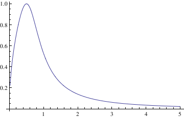
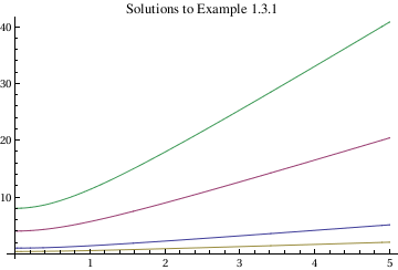
Plot[{Sqrt[1 + x*x], 4*Sqrt[1+x*x], 0.4*Sqrt[1+x*x], 8*Sqrt[1+x*x]}, {x, 0, 5}, PlotLabel -> "Solutions to Example 1.3.1 "]
In this command sequence, the first line of code asks Mathematica to find the solution to this separable differential equation.
The second line contains commands to plot different possible solutions to this separable differential equation based on the value of the integration constants. None of the subcommands of Plot are new in this command sequence and they have already been explained earlier.
The second method for solving the separable differential equations is to use Mathematica to solve the equation by direct integration and to then plot those solutions:
Clear[t,y];
t0 = 0; y0 = 2; f[t_] = t/(1 + t^2); g[y_] = 1/y; (* define the initial values and the slope functions *)
F[t_] = Integrate[f[t], t]; G[y_] = Integrate[g[y], y];
gensol = Solve[G[y] == F[t] + c, y];
const = Solve[y == y0 /. gensol /. t -> t0, c];
sol[t_] = y /. gensol /. const[[1]] (* solution of the IVP *)
Out[6] = {2 Sqrt[1 + t^2]}
Plot[sol[t], {t, -2, 2}]
In this syntax, the first command, Clear, clears out any previously existing values for the two variables, allowing you to redefine them.
The second command defines the different initial conditions and the two functions that you are trying to solve.
The first command line tells Mathematica which functions you want to integrate.
The fourth and fifth lines tell Mathematica how you want to define the general solution and how you want to solve for the integration constant c.
The sixth line gives the final solution to this separable differential equation (this is also an initial value problem).
The final line tells Mathematica which function to plot and the range.
In Mathematica, as this example shows, you can insert comments to the commands by adding a comment surrounded by stars and then parentheses.
Example 2.3.2. Consider separable differential equation: y' +ycos(x) =0
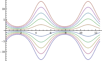
sol = DSolve[y'[x] == -Cos[x]*y[x], y[x], x]
Out[1]= {{y[x] -> E^-Sin[x] C[1]}}
toplot = Table[E^-Sin[x] C[1] /. C[1] -> i, {i, -5, 5}];
Plot[Evaluate[toplot], {x, 0, 4*Pi}]
Example 2.3.3. Consider separable differential equation: x(y+1)(y-3) dx +(1+5y)(x+2) dy =0. We solve this equation by separating variables and then integrating:
Integrate[x/(x + 2), x] + Integrate[(1 + 5*y)/(y + 1)/(y - 3), y] == c
Out[1] = x - 2 Log[2 + x] + 4 Log[-3 + y] + Log[1 + y] == c
solution = E^x *(x + 2)^(-2) * (y - 3)^4 *(1 + y)
Out[2] = (E^x (-3 + y)^4 (1 + y))/(2 + x)^2
factored = Factor[Dt[solution]] /. {Dt[x] -> dx, Dt[y] -> dy}
Out[3] = (E^x (-3 + y)^3 (2 dy - 3 dx x + dy x + 10 dy y - 2 dx x y +
5 dy x y + dx x y^2))/(2 + x)^3
diffExpr = Collect[factored[[4]], {dx, dy}]
Out[4] = dy (2 + x + 10 y + 5 x y) + dx (-3 x - 2 x y + x y^2)
dxPart = Factor[Coefficient[diffExpr, dx]]
Out[5] = x (-3 + y) (1 + y)
dyPart = Factor[Coefficient[diffExpr, dy]]
Out[6] = (2 + x) (1 + 5 y)
dxPart*dx + dyPart*dy == 0
Out[7] = dx x (-3 + y) (1 + y) + dy (2 + x) (1 + 5 y) == 0
We present several classes of equations that can be reduced to a separable one. We start with the differential equation of the form
\[
y' = F(ax +by +c), \qquad b\ne 0,
\]
where \( F(v) \) is a given continuous function of a variavle variable v, and a,b,c are some constants. This equation is reduced to a
separable one by substitution \( v=ax+by +c . \)
Another class of equations is
\[
x\,y' = y\,F(xy),
\]
where F(v) is a function of the product v=xy.
Our next class includes differential equations with homogeneous coefficients when the clope function is a function depending on the ration y/x:
\[
y' = F(y/x) .
\]
This equation is reduced to a separable one by substitution v=y/x or y = xv.
Example 2.4.1.
First, we find solutions to the equation \( xy'=x^2 y^3 -y/x \) using the standard Mathematica command:
DSolve[y'[x] == x*(y[x])^3 -y[x]/x,y[x],x]
and then plot solutions:
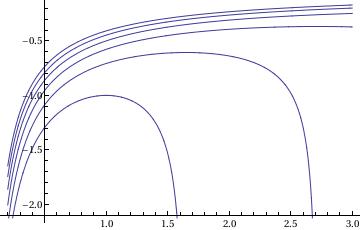
solution = DSolve[y'[x] == x*(y[x])^3 - y[x]/x, y[x], x]
g[x_] = y[x] /. solution[[1]]
t[x_] = Table[g[x] /. C[1] -> j, {j, 1, 6}]
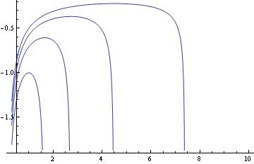
Plot[t[x], {x, 0.2, 3}]
Example 2.4.2.
Reduction of the equation y' =-(x^2 + y^2)/(5xy) to a separable equation. We answer this question using Mathematica:
ode[x_, y_] = -(x^2 + y^2)*dx == 5*x*y*dy
Out[8] = dx (-x^2 - y^2) == 5 dy x y
ode[x, v*x] /. {dy -> x*dv + v*dx}
Out[9] = dx (-x^2 - v^2 x^2) == 5 v x^2 (dx v + dv x)
Map[Cancel, Map[Function[q, q/x^2], %]]
Out[10] = -dx (1 + v^2) == 5 v (dx v + dv x)
Map[Function[u, Collect[u, {dx, dv}]], %]
Out[11] = -dx (1 + v^2) == 5 dx v^2 + 5 dv v x
Example 2.4.3.
We consider the differential equation with homogeneous slope function
\[
y' = \frac{y-x}{y+x} = \dfrac{y/x -1}{y/x +1} .
\]
Making change of depending variable
\( y/x =v \) or
\( y(x) = x\,v(x) , \) we obtain a separable equation in variable v:
\[
y' = v(x) + x\,v' (x) = \frac{v-1}{v+1} \qquad\Longrightarrow \qquad x\,v' = \frac{v-1}{v+1} -v = - \frac{v^2 +1}{v+1} .
\]
Separation of variables yields
\[
\frac{v+1}{v^2 +1}\,{\text d}v = - \frac{{\text d}x}{x} \qquad\Longrightarrow \qquad \arctan v + \frac{1}{2}\,\ln (v^2 +1 ) = \int \frac{v+1}{v^2 +1}\,{\text d}v = - \int \frac{{\text d}x}{x} = -\ln Cx .
\]
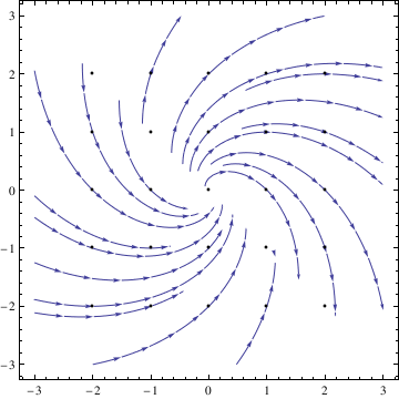
points := Tuples[{-2, -1, 0, 1, 2}, 2]
Table[StreamPlot[{1, {(y - x)/(x + y)}}, {x, -3, 3}, {y, -3, 3},
StreamPoints -> {points, Automatic, maxlen},
Epilog -> Point[points]], {maxlen, {2.5, Scaled[.05]}}]
Example 2.4.4. Consider the initial value problem
y' = 1/(x-y+2), y(0) =1 .
We find its solution (in implicit form) and plot it using the following Mathematica commands:
ans1 = DSolve[{y'[x] == 1/(x - y[x] + 2), y[0] == 1}, y[x], x]
Plot[y[x] /. ans1, {x, -1, 1}, PlotRange -> {0, 2}, AspectRatio ->1]
ans2 = DSolve[{x'[y] == x[y] - y + 2, x[1] == 0}, x[y], y] //Simplify
ParametricPlot[Evaluate[{x[y], y} /. ans2], {y, 0, 2},
PlotRange -> {{-1, 1}, {0, 2}}, AspectRatio -> 1]
Example 2.4.5.
Another example.
eq = 2 x^2 + y^2 - 2 x y + 5 x == 0
Out[1]= 5 x + 2 x^2 - 2 x y + y^2 == 0
step1= Dt[eq,x]
Out[2]= 5 + 4 x - 2 y - 2 x Dt[y, x] + 2 y Dt[y, x] == 0
step2=Solve[step1,Dt[y,x]]
Out[3]= {{Dt[y, x] -> (5 + 4 x - 2 y)/(2 (x - y))}}
To extract the left-hand side, type:
eq[[1]]
Out[4]= 5 x + 2 x^2 - 2 x y + y^2
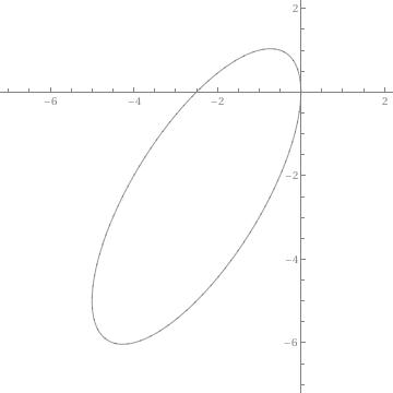
Then we plot the graph:
ContourPlot[Evaluate[eq[[1]]], {x, -7, 2}, {y, -7, 2}, Frame -> False,
Axes -> Automatic, AxesOrigin -> {0, 0},
AxesStyle -> GrayLevel[0.5], PlotPoints -> 100, Contours -> {0},
ContourShading -> False]
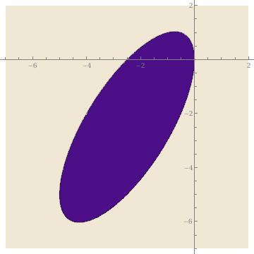
If the option
ContourShading
is removed, we will get
In the above graphs, the option Contour->{0} instructs
Mathematica to graph only the level curve corresponding to 0.
The option
ContourShading -> False
specifies to not shade the regions between contours,
Frame -> False
specifies that a frame is not to be placed around the
resulting graphics objects,
Axes -> Automatic
specifies that axes are to be placed on the resulting
graphics objects while the option
AxesOrigin -> {0, 0}
specifies that they intersect at the point (0,0), and the option
AxesStyle -> GrayLevel[0.5]
specifies that they be drawn in a medium shade of gray.
The option
PlotPoints -> 100
instructs
Mathematica to increase the number of sample points to 100 (the default is 15), elping assure that the resulting graphic object appears smooth.
Note that instead of
eq[[1]], one can use the equation 5 x + 2 x^2 - 2 x y + y^2 explicitely.
Example 2.4.6.
Consider the differential equation
dy/dx = ( (2x-2y-2) / {x-1})^2 , where x != 1
We exclude the singular point x=1 where the
integral curves have an infinite slope. The right-hand side
function (= slope function) is a composition of two functions:
( (2x-2y-2) / (x-1) )^2 = F(z(x,y)) , where F(z) = z^2 and z = (2x-2y-2) / (x-1) .
The function F(z(x,y)) is not homogeneous, but it can be converted to a homogeneous one by shifting
\( x=X+\alpha \) and \( y=Y+\beta ,\)
where
\( \alpha = 1, \) \( \beta = 0 \)
so \( x=X+1, \ y=Y.\) We next substitute \( x=X+1 \) and \( y=Y \) into the given
equation and simplify. The result is
\[
\text{d}Y/\text{d}X = \text{d}y / \text{d}(x-1) = \text{d}y /\text{d}x = (2(x-1)
-2y/{x-1} )^2 = ( (2X -2Y) / X )^2
\]
Setting \( Y=vX \) gives us
\[
X \text{d}v /\text{d}X +v = 4 (1-v)^2 \qquad \mbox{or} \qquad \text{d}v (4(1-v)^2 -v) = \text{d}X / X .
\]
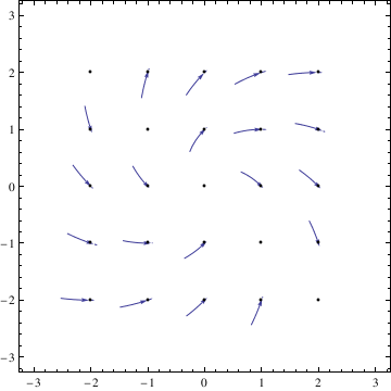
Plotting the direction field, it can be seen that \( v = a /2 \approx 1.64039 \) is unstable equilibrium solution, and \( v=
\frac{b}{2} \approx 0.609612 \) is a stable equilibrium solution. These
critical points are not singular solutions because integral curves do
not touch them, which means that an initial value problem for the
differential equation \( X\,v' = (2v-a)(2v-b) \) has a unique solution.
Now we return to the original variables. Since \( X=x-1, \ Y=y \), and
\( v=Y/X, \) the original differential equation has the general solution
in implicit form:
\[
C|x-1|^{\sqrt{17}} = \left| \frac{8y -(9 + \sqrt{17})(x-1)}{8y -(9 -\sqrt{17})(x-1)} \right| , \qquad x \ne 1.
\]
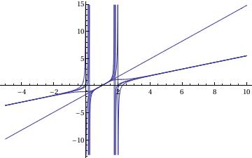
It can be solved with respect to \( y, \) and then plotted using the following Mathematica commands:
a:=Abs[Sqrt[17]]; Plot[((x - 1)*(#1 Abs[x - 1]^a *(9 - a) - 9 - a)/(#1 Abs[x - 1]^a - 1)/ 8 &) /@ {-1, 0, 1, 2, 3}, {x, -5, 10}]
The given differential equation has two equilibrium solutions that correspond to \( v=a/2 \) and \( v=b/2 \):
\[
y = (x-1) a/2 = (x-1) (9+\sqrt{17) )/8 and
y = (x-1) b/2 = (x-1) (9-\sqrt(17)) /8.
\]
The equation \( y \,\text{d}x + x \,\text{d}y =0 \) is exact. Consider the initial condition \( y(2)=3 \)
Since Mathematica uses the command "N" for numerical evaluation, we change notation \( M(x,y) \,\text{d}x + N(x,y)\, \text{d}y =0 \) as
\( MM(x,y) \) and \( NN(x,y) \)
MM[x_, y_] = y;
NN[x_, y_] = x;
{p1, p2} = {2, 3};
Simplify[D[MM[x, y], y] == D[NN[x, y], x]]
Out[4] = True
psi[X_, Y_] =
Integrate[MM[x, p2], {x, p1, X}] + Integrate[NN[X, y], {y, p2, Y}]
Out[22]= 3 (-2 + X) + X (-3 + Y)
The solution is psi[x,y]==0:
Define the gradient function:
grad[potential_, vars_List] := Map[Function[t, D[potential, t]], vars]
and then check our potential function:
grad[psi[x, y], {x, y}]
Out[25]= {y,x}
Example 2.5.1.
MM=x+2 y; NN=2 x-3 y;
a=TrueQ[D[MM,y]==D[NN,x]];
If[a==True, Print["The equation is exact"], Print["The equation is not exact"]]
Out[4] = The equation is exact
F = Integrate[MM,x]
Out[5] = x^2/2 + 2 x y
derfy = D[F, y] - NN
Out[6] = 3 y
f[y] = Integrate[derfy, y]
Out[7] = (3 y^2)/2
psi = F + f[y]
Out[8] = x^2/2 + 2 x y + (3 y^2)/2
Print["psi=", psi];
Out[9] = psi=x^2/2+2 x y+(3 y^2)/2
Print["Trajectories of psi..."]
Out[10] = Trajectories of psi...
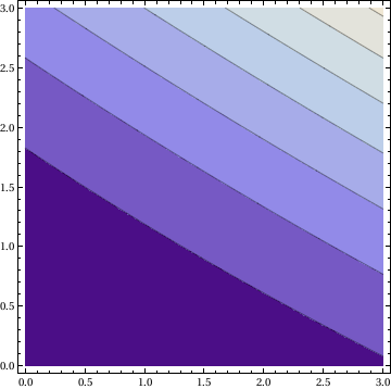
ContourPlot[F,{x,0,3},{y,0,3}]

Example 2.6.1. The equation
\[
x(y^2 +y-6) \,\text{d}x (x-3)(1+2y) \,\text{d}y=0
\]
is separable, with integrating factor
\( \mu(x,y)=(x-3)^(-1) (y^2 +y -6)^(-1). \)
Then we integrate
Integrate[x/(x - 3), x] +
Integrate[(1 + 2*y)/((y + 3)*(y - 2)), y] == C
Out[31]= x + 3 Log[-3 + x] + Log[-6 + y + y^2] == C
After exponentiating, we get
e^x (x-3)^3 (y^2 + y-6) =e^C = c (* which we denote by c *)
Now we check with the following steps:
solution = Exp[x] (x - 3)^3 (y^2 + y - 3)
Out[31] = E^x (-3 + x)^3 (-3 + y + y^2)
factored = Factor[Dt[solution]] /. {Dt[x] -> dx, Dt[y] -> dy}
Out[33]= E^x (-3 + x)^2 (-3 dy - 3 dx x + dy x - 6 dy y + dx x y + 2 dy x y + dx x y^2)
diffExpression = Collect[factored[[3]], {dx, dy}]
Out[34] = dy (-3 + x - 6 y + 2 x y) + dx (-3 x + x y + x y^2)
dxPart = Factor[Coefficient[diffExpression, dx]]
Out[35] = x (-3 + y + y^2)
dyPart = Factor[Coefficient[diffExpression, dy]]
Out[36] = (-3 + x) (1 + 2 y)
dxPart*dx + dyPart*dy == 0
Out[37]= dy (-3 + x) (1 + 2 y) + dx x (-3 + y + y^2) == 0
A linear differential equation is an equation of the form:
\[
y' + a(x) y = f(x) .
\]
is called the
linear equation, where f(x) is the forcing, input or nonhomogeneous part. The equation
\[
y' + a(x) y = f(x)\, y^p , \qquad\mbox{where} \quad p \ne 0, 1 .
\]
is referred to as the
Bernoulli equation. Both equations, linear and Bernoulli, can be solved using the Bernoulli substitution:
\[
y(x) = u(x)\,v(x) ,
\]
where
\( u(x) \) is a solution of truncated separable equation
\[
u' + a(x) \,u = 0 , \qquad\Longrightarrow \qquad u(x) = \exp \left\{ -\int a(x)\,{\text d}x \right\} .
\]
Then function
\( v(x) \) is a solution of the separable equation
\[
u\, v' = f(x) \, u^p v^p ,
\]
where p=0 for the linear equation.
Example 2.7.1.
ode[x_,y_] = (y'[x] - 5 y[x] == 0)
SolRule = DSolve[ode[x, y], y[x], x]
yh[x_] = Simplify[y[x] /. SolRule[[1]]] (* solution of the homogeneous eq *)
Simplify[ode[x, yh]] (* to check the answer *)
Nonhomogeneous equation:
nde[x_, y_] = (y'[x] - 5 y[x] == 27 x^3 Exp[2 x])
SolnRule = DSolve[nde[x, y], y[x], x]
yn[x_] = Simplify[y[x] /. SolnRule[[1]]]
Out[11]= -E^(2 x) (2 + 6 x + 9 x^2 + 9 x^3) + E^(5 x) C[1]
It can be obtained in one line:
yn[x_] = Simplify[(y[x] /. DSolve[nde[x, y], y[x], x][[1]])]
Example 2.7.2. Another example:
SolxRule = DSolve[x y'[x] - 5 y[x] == 27 x^7 * Exp[x], y[x], x]
y3[x_] = Simplify[y[x]/.SolxRule[[1]]]
Out[11]= x^5 (27 E^x (-1 + x) + C[1])
Checking:
Simplify[x y3'[x] -5 y3[x] == 27 x^7 * Exp[x]]
Example 2.7.3. Solve the IVP: \( 3ty' +2y=t^2 , y(1)=1 \)
Clear[t, y];
t0 = 1; y0 = 1;
p[t_] = 2/3/t; q[t_] = t/3;
P[t_] = Exp[Integrate[p[s], {s, t0, t}]];
y[t_] = 1/P[t]*(t0 + Integrate[P[u]*q[u], {u, t0, t}])
Out[2]= ConditionalExpression[ConditionalExpression[(1 + 1/8 (-1 + t^(8/3)))/t^(2/3), Re[t] >= 0 || t \[NotElement] Reals],
(Re[t] >= 0 || t \[NotElement] Reals) && (Re[u] >= 0 || u \[NotElement] Reals)]
Example 2.7.4. Solve the IVP:
Clear[x,y,gensol] (* clear all variables *)
gensol=DSolve[y'[x]==Exp[-2 x]-3 y[x],y[x],x]
Out[11]= {{y[x] -> E^(-2 x) + E^(-3 x) C[1]}}
gensol[[1,1,2]]
Out[12]= E^(-2 x) + E^(-3 x) C[1]
In DSolve command, the first argument (y'[x]==Exp[-2 x]-3 y[x]) represents the differential equation,
the second argument (y[x]) instructs Mathematica that we are solving for y=y(x), and
the thrid argument (x) instructs Mathematica that the independent variable is x.
Note that gensol is a nested list. The first part of gensol, extracted with gensol[[1]], is the list (y(x)->E^(-2 x) + E^(-3 x) C[1]);
and the first part of this list, extracted with gensol[[1,1,1]], is y(x) while the second part of this list
(which represents the formula for the solution), extracted with gensol[[1,1,2]], is y=E^(-2 x) + E^(-3 x) C[1]
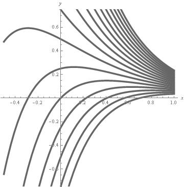
toplot=Table[(gensol[[1,1,2]])/.C[1]->i,{i,-2,2,0.25}];
pp=Plot[Evaluate[toplot],{x,-1/2,1},PlotRange->{-3/4,3/4},AspectRatio->1,
AxesStyle->GrayLevel[0.5],PlotStyle->{{GrayLevel[0.4],Thickness[0.01]}}, AxesLabel->{x,y}]
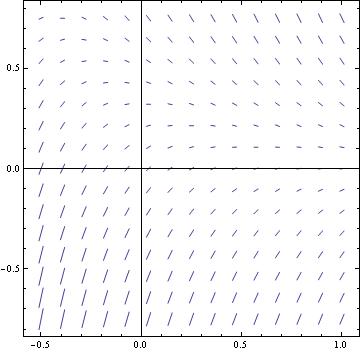
pd = VectorPlot[{1, Exp[-2 x] - 3 y}, {x, -1/2, 1}, {y, -3/4, 3/4},
Axes -> Automatic, VectorScale -> (1 &), AxesOrigin -> {0, 0}, VectorStyle -> Arrowheads[0]]
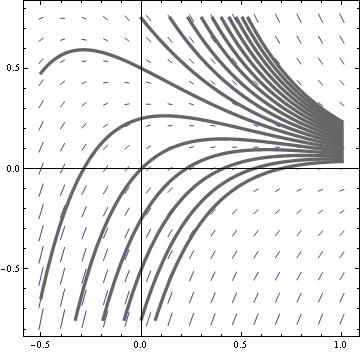
Show[pd, pp]
To solve the Bernoulli equation x' +px=qy^n , we use substitution
y=x^(1-n)
L[x_] := D[x, t] + p*x - q*x^n;
x = y[t]^(1/(1 - n));
a2 = Simplify[L[x]];
a3 = a2/y[t]^(n/(1 - n));
Simplify[PowerExpand[a3]]
Out[36]= ConditionalExpression[
8^(n/(1 - n)) t^((2 n)/(3 - 3 n)) (7 + t^(8/3))^(
n/(-1 + n)) (p (7/(8 t^(2/3)) + t^2/8)^(1/(1 - n)) -
q (7/(8 t^(2/3)) + t^2/8)^(n/(1 - n)) - (
2 (7/(8 t^(2/3)) + t^2/8)^(1/(1 - n)) (-7 + 3 t^(8/3)))/(
3 (-1 + n) t (7 + t^(8/3)))), (Re[t] >= 0 ||
t \[NotElement] Reals) && (Re[u] >= 0 || u \[NotElement] Reals)]
Give codes using the Bernoulli method: x=u*v, where u' +p*u=0 and v is the solution of the separable equation uv' =(u*v)^n
Example 2.7.5.
The four streamlines (corresponding to the values of an arbitrary constant C=1,2,3,4) from the general solution y=1/(x Sqrt[C-2 ln[x]]) of the Bernoulli equation
x y' =x^2 y^3 -y can be plotted with one command:
Plot[-1/(x Sqrt[#1 - 2 Log[x]] &) /@ {1, 2, 3, 4}, {x, .3, 10} ]
Example 2.7.6. Example
y y' =y^2 +e^x
The general solution: y=\pm Sqrt[c e^(2x)-2 e^x] , where c is an arbitrary constant.
curves = Flatten[
Table[{Sqrt[-2 E^x + c E^(2 x)], -Sqrt[-2 E^x + c E^(2 x)]}, {c,
1/4, 3, 3/4}]] (* increament is 3/4 *)
Out[1]= {Sqrt[-2 E^x + E^(2 x)/4], -Sqrt[-2 E^x + E^(2 x)/4], Sqrt[-2 E^x +
E^(2 x)], -Sqrt[-2 E^x + E^(2 x)], Sqrt[-2 E^x + (7 E^(2 x))/
4], -Sqrt[-2 E^x + (7 E^(2 x))/4], Sqrt[-2 E^x + (5 E^(2 x))/
2], -Sqrt[-2 E^x + (5 E^(2 x))/2]}
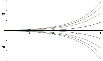
Plot[Evaluate[curves], {x, 0, 4}, PlotRange -> All]
Example 2.7.7. Example
y' +xy=x y^4
BerEq[x_,y_] := D[y[x],x]+x y[x] == y[x]^4
BNum =4
u[x_] == y[x]^(1-BNum)
yp = Solve[u'[x] == D[y[x]^(1-BNum),x],y'[x]]
LeftSide = Map[Function[t, t/y[x]^BNum],
BerEq[x, y] /. yp[[1]] /. {(a_ == b_) -> a - b}]
L[x_, u_] = LeftSide /. {y[x]^(1 - BNum) -> u[x]}
SolU = DSolve[L[x,u] == 0,u[x],x]
Sol[x_] = Simplify[(u[x]/.SolU[[1]]^(1/(1-BNum)))]
Out[4]= 4
Out[5]= u[x_] == 1/y[x]^3
Out[6]= {{Derivative[1][y][x] -> -(1/3) y[x]^4 Derivative[1][u][x]}}
Out[7]= -1 + x/y[x]^3 - Derivative[1][u][x]/3
Out[8]= -1 + x u[x] - Derivative[1][u][x]/3
Out[9]= {{u[x] ->
E^((3 x^2)/2) C[1] -
E^((3 x^2)/2) Sqrt[(3 \[Pi])/2] Erf[Sqrt[3/2] x]}}
Out[10]= u[x] /. {1/(u[x] ->
1/2 E^((3 x^2)/2) (2 C[1] - Sqrt[6 \[Pi]] Erf[Sqrt[3/2] x]))^(1/3) }
Example 2.8.1.
Consider the Riccati equation
\[
y' = 2y/x+y^2 -x^4 .
\]
It can be solved by substitution y =x^2 +1/v(x) , where y1=x^2 is a particular solution of the given Riccati equation.
R[x_, y_] = (y'[x] - 2 y[x]/x - y[x]^2 + x^4 )
y1[x_] = x^2
R[x, y1]
Simplify[Expand[v[x]^2 R[x, Function[t, t + t/v[t]]]]]
DSolve[% == 0, v[x], x] (* solve linear equation for v *)
y2[x_] = Simplify[(y1[x] + 1/v[x]) /. %[[1]]]
Out[11]= x^4 - (2 y[x])/x - y[x]^2 + Derivative[1][y][x]
Out[12]= x^2
Out[13]= 0
Out[14]= -(1 + 2 x^2) v[x] + (-1 - x^2 + x^4) v[x]^2 - x (x + Derivative[1][v][x])
Out[15]= {{v[x] -> -(x (-(E^((2 x^3)/3 - 1/6 x^2 (3 + 2 x))/(2 x)) + (
E^((2 x^3)/3 - 1/6 x^2 (3 + 2 x)) (1 + x))/(2 x^2) - (
E^((2 x^3)/3 - 1/6 x^2 (3 + 2 x)) (1 + x) ((5 x^2)/3 - 1/3 x (3 + 2 x)))/(
2 x) + (-((E^(-(1/6) x^2 (3 + 2 x)) (-1 + x))/x^2) +
E^(-(1/6) x^2 (3 + 2 x))/x + ( E^(-(1/6) x^2 (3 + 2 x)) (-1 + x) (-(x^2/3) -
1/3 x (3 + 2 x)))/x) C[1]))/((-1 - x^2 + x^4) (-((E^((2 x^3)/3 - 1/6 x^2 (3 + 2 x)) (1 + x))/(
2 x)) + (E^(-(1/6) x^2 (3 + 2 x)) (-1 + x) C[1])/x))}}
Out[16]= (E^((2 x^3)/3) (-1 - x + x^2) + 2 (-1 + x + x^2) C[1])/(E^((
2 x^3)/3) + 2 C[1])
Example Clairaut Equation
y=xy' + (y')^2
Clear[y];
y[x_] = x c + c^2
samples =Table[y[x],{c,-3,3,1/4}]
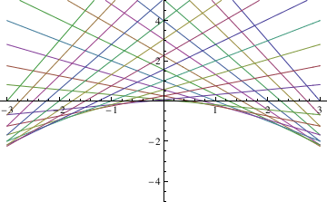
Plot[Evaluate[samples],{x,-3,3},PlotRange->{-5,5}]
Out[18]= c^2 + c x
Out[19]= {9 - 3 x, 121/16 - (11 x)/4, 25/4 - (5 x)/2, 81/16 - (9 x)/4, 4 - 2 x,
49/16 - (7 x)/4, 9/4 - (3 x)/2, 25/16 - (5 x)/4, 1 - x,
9/16 - (3 x)/4, 1/4 - x/2, 1/16 - x/4, 0, 1/16 + x/4, 1/4 + x/2,
9/16 + (3 x)/4, 1 + x, 25/16 + (5 x)/4, 9/4 + (3 x)/2,
49/16 + (7 x)/4, 4 + 2 x, 81/16 + (9 x)/4, 25/4 + (5 x)/2,
121/16 + (11 x)/4, 9 + 3 x}
Out[20]=
To find the singular solution (envelope), we type:
f[t_] = t^2;
Eliminate[{x==-f'[t],y==f[t]-t*f'[t]},t]
Out[37]= -4y==x^2
Example 2.11.1. (Orthogonal trajectories)
Given the family of curves x*y=c, where c is a constant. These are
hyperbolas in quadrants 1 and 3 for c>0 or quadrants 2 and 4 for c<0,
having the axes as asymptotes. They are rectengular hyperbolas
because their asymptotes are perpendicular. The differential equation
of the family is x y' + y =0, or dy/dx = -y/x . The orthogonality
condition says that the equation of the orthogonal curves should be -
dx/dy = -y/x or dy/dx = y/x . The latter has the general solution
(after separation of variables): y^2 = x^2 +c. Now we plot these
curves.
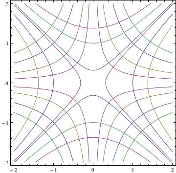
a := ContourPlot[{x y == 1, x y == 0.2, x y == 0.5, x y == 1.5,
x y == -1, x y == -0.2, x y == -0.5, x y == -1.5}, {x, -2, 2}, {y, -2, 2}]
b := ContourPlot[{x^2 == y^2 + 1, x^2 == y^2 + 0.1, x^2 == y^2 + 1.9,
x^2 == y^2 - 1, x^2 == y^2 - 0.1, x^2 == y^2 - 1.9}, {x, -2, 2}, {y, -2, 2}]
Show[a, b]
Example 2.11.2.
The differential equation Exp[y] dy = Sin[x] dx defines its
family of solutions: Exp[y] == Sin {x] +c .
The orthiogonal trajectories are ln | Tan[x/2] = Exp[y] +c.
a := ContourPlot[{Exp[y] + Cos[x] == 3, Exp[y] + Cos[x] == 0.2,
Exp[y] + Cos[x] == 2, Exp[y] + Cos[x] == 0.5,
Cos[x] + Exp[y] == 1.5, Cos[x] + Exp[ y] == -2,
Cos[x] + Exp[y] == -0.2, Cos[x] + Exp[ y] == -0.5,
Cos[x] + Exp[y] == -1.5}, {x, -2, 2}, {y, -2, 2}]
b := ContourPlot[{Log[Tan[x]] == Exp[-y] + 1,
Log[Tan[x]] == Exp[-y] + 0.1, Log[Tan[x]] == Exp[-y] + 0.9,
Log[Tan[x]] == Exp[-y] - 1, x Log[Tan[x]] == Exp[-y] - 0.1,
Log[Tan[x]] == Exp[-y] - 3.9}, {x, -2, 2}, {y, -2, 2}]
Show[a, b]
>>>>> ortho2.jpg
Example 2.11.3. (Logistic equation)
The logistic equation can be solved and plotted as follows.
LogisticEquation = y'[t] == r (1 - (y[t]/k))*y[t] - h*y[t];
DSolve[LogisticEquation, y, t]
Out[1]=
{{y -> Function[{t}, -((E^(r t + h k C[1]) k (-h + r))/(
E^(h t + k r C[1]) - E^(r t + h k C[1]) r))]}}
sol = DSolve[{LogisticEquation /. {r -> (1/2), k -> 10, h -> (1/4)}, y[0] == a}, y, t]
Out[2]=
{{y -> Function[{t}, (5 a E^(t/4))/(5 - a + a E^(t/4))]}}
To plot the results, we employ two options:
tab = Table[y[t] /. sol[[1]] /. {a -> k}, {k, -5, 5}]
Out[3]=
{-((25 E^(t/4))/(10 - 5 E^(t/4))), -((20 E^(t/4))/(
9 - 4 E^(t/4))), -((15 E^(t/4))/(8 - 3 E^(t/4))), -((10 E^(t/4))/(
7 - 2 E^(t/4))), -((5 E^(t/4))/(6 - E^(t/4))), 0, (5 E^(t/4))/(
4 + E^(t/4)), (10 E^(t/4))/(3 + 2 E^(t/4)), (15 E^(t/4))/(
2 + 3 E^(t/4)), (20 E^(t/4))/(1 + 4 E^(t/4)), 5}
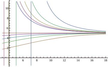
Plot[Evaluate[tab], {t, 3, 18}]
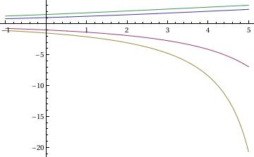
Plot[Evaluate[
y[t] /. sol /. {{a -> 1}, {a -> -1}, {a -> -1.5}, {a ->
1.5}}], {t, -1, 5}, PlotRange -> All]
Some parts of the syntax of the code may be confusing, so that will
be explained here.
You may wonder why the variable x[k] and y[k] are used instead of x(k)
and y(k). The reason is because the brackets [] resemble the denotation
you see. Therefore, x[k] and y[k] in actual form would be xk and yk
respectively. The parenthesis, on the other hand, would resemble the
independent variable relevant to the dependent variable in the
parenthesis.
Martha L. Abell, James P. Braselton
Differential Equations With Mathematica,
Academic Press, 2004
ISBN 0120415623, 978012041562
Alfred Gray, Mike Mezzino, and Mark Pinsky
Introduction to Ordinary Differential Equations with Mathematica: An Integrated Multimedia Approach
Springer
ISBN-10: 0387944818 | ISBN-13: 978-0387944814
Brian R. Hunt, Ronald L. Lipsman, John E. Osborn, Donald A. Outing, Jonathan Rosenberg
Differential Equations with Mathematica, 3rd Edition
ISBN: 978-0-471-77316-0
Clay C. Ross
Differential Equations
An introduction with Mathematica
Springer-Verlag, 1995
ISBN: 0-387-94301-3
