Second and Higher Order Differential Equations
This tutorial contains many Mathematica scripts. You, as the user, are free to use all codes for your needs, and have the right to distribute this tutorial and refer to this tutorial as long as this tutorial is accredited appropriately. Any comments and/or contributions for this tutorial are welcome; you can send your remarks to <Vladimir_Dobrushkin@brown.edu>
Return to computing page for the second course APMA0330
Return to Mathematica tutorial page for the first course
Return to Mathematica tutorial page for the second course
Return to the main page for the course APMA0330
Return to the main page for the course APMA0340
Content
Part IV. Second and hifger order differential equations
Fundamental set of solutions. Wronskian
General solution
Reduction of order
Non-homogeneous equations.
Lagrange's method
Method of undetermined coefficients
Operator methods (not sure yet)
Numerical Solutions of second order ODEs
Applications
1.4.1. Fundamental Set of Solutions
To check linearly independence of two functions, we have two options. First, two functions are linearly independent if and only if one of them is a constant multiple of another. Another option is to calculate the Wronskian if you know that these two functions are solutions of the same differential equation.
Example. Given two functions \( \{ x , 3x \} ,\) determine whether they are linearly dependent.
w={y,D[y,x]}
Det[w]
I. Wronskian
The Mathematica command Wronskian[{y1 ,y2, ...},x] gives the Wronskian determinant for the functions \( y1 (x), y2 (x) , \ldots ,\) depending on x.
1.4.2. General Solutions of Homogeneous Equations
I. Verification
Example 4.4.1. We verify that the function \( y(x) = C_1 \,\cos 2x + C_2 \,\sin 2x + x^3 -3x/2 \) is a solution of the differential equation \( y'' + 4\,y = 4\,x^3 .\)
Simplify[y''[x] + 4 y[x] == 4 x^3]
c1c2 = Solve[ics, {c1, c2}];
SolRule[x_] = y[x] /. c1c2[[1]]
SolRule''[x] + 4 SolRule[x] == 4 x^3 && SolRule[0] == 1 && SolRule'[0] == -1
Simplify[%]
To check linearly dependence:
y={Cos[2 x], Sin[2 x]}
w={y,D[y,x]}
Det[w]
w={y,D[y,x]}
Det[w]
Example 4.4.2. We consider the linear differential operator:
II. Linear Differential Operators
L[x_,y_] =y''[x] -y'[x]- 6y[x]
CharPoly[lambda_] =Coefficient[L[x,Exp[lambda #]&], Exp[lambda x]]
roots =lambda/.Solve[CharPoly[lambda]==0,lambda]
AllSoln[x_]=Soln.{c1,c2}
Higher Order Equations
char[lambda_] =Coefficient[L[x,Function[t,Exp[lambda t]]],Exp[lambda x]]
roots = r /. Solve[char[r] == 0, r]
solns = Map[Function[k, Exp[k x]], roots]
y[x_] = solns.{c2,c1,c3} (* or *)
Clear[x,y];
L[x_, y_] = y'''[x] - 2 y''[x] - 5 y'[x] + 6 y[x]
DSolve[L[x, y] == 0, y[x], x]
y[x_] = Expand[y[x] /. %[[1]] ]
basis = Table[Coefficient[y[x], C[i]], {i, 1, 3}]
Factor[Coefficient[L[x, Function[t, Exp[r t]]], Exp[r x]]]
W[x_] = NestList[Function[t, D[t, x]], basis, 2]
Det[W[x]]
Composition of Linear Differential Operators:
L3[x_, y_] := b[3] D[y[x], {x, 3}] + b[2] D[y[x], {x, 2}] + b[1] D[y[x], {x, 1}] + b[0] y[x]
L2L3 = Collect[L2[x, Function[z, L3[z, y]]], y]
III. Real Distinct Roots
IV. Complex Roots
w = {y, D[y, x]};
Det[w] (* or *)
Simplify[Det[w], Trig -> True]
IVP:
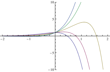
soln[x_] = Expand[y[x] /. %[[1]]] /. C[1] -> c1
curves = Table[soln[x], {c1, -2, 2}];
Plot[Evaluate[curves], {x, -2, 2}, PlotRange -> {-10, 10}]
Out[13]=
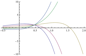
soln[x_] = Expand[y[x] /. %[[1]]] /. C[1] -> c2
curves = Table[soln[x], {c2, -2, 2}];
Plot[Evaluate[curves], {x, -0.5, 2}, PlotRange -> {-10, 10}]
Out[17]=
Example.
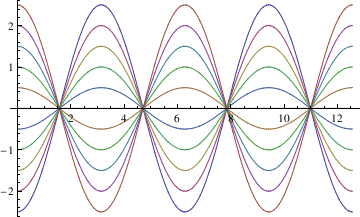
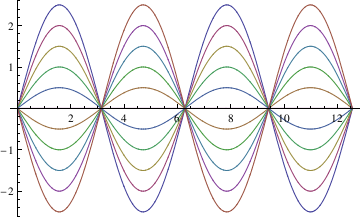
Consider the second order differnetial equation \( y'' +y=0, \) which has two linearly independent solutions:
\( \cos x, \sin x .\)
Table[C[2] Cos[x] - C[1] Sin[x] /. {C[2] -> i, C[1] -> 0}, {i, -2.5, 2.5, 0.5}];
Table[C[2] Cos[x] - C[1] Sin[x] /. {C[2] -> 0, C[1] -> i}, {i, -2.5, 2.5, 0.5}];
plot1 = Plot[Evaluate[toplot1], {x, 0, 4*Pi},
DisplayFunction -> Identity]
V. Boundary Value Problem
yb[x_] = y[x] /. DSolve[L[x, y] == 36 x, y[x], x][[1]]
const = Solve[{yb[0] == 2, yb[1] == 1, yb[2] == -1}, {C[1], C[2], C[3]}]
z[x_] = Simplify[yb[x] /. const[[1]]]
E^2 + E^3 + E^4)) + ( E^(-1 + x) (-10 + 18 E^2 + 3 E^3 - 10 E^5))/((-1 + E)^2 (1 + E) (1 +
E + E^2)) + (E^(4 - 2 x) (-18 + 10 E + 10 E^3 - 3 E^4))/(
1 - E^3 - E^5 + E^8) + 6 x
zb[x_] = yb[x] /. {C[1] -> p1, C[2] -> p2, C[3] -> p3}
Plot[zb[x], {x, -1, 2.5}]
1.4.3. Reduction of Order
I. Double Roots
soln[x_] = Expand[y[x]/.%[[1]]]
y1[x_] = Coefficient[soln[x],C[1]]
y2[x_] = Coefficient[soln[x], C[2]]
basis = {y1[x], y2[x]}
WronskianDet = Det[{basis, D[basis, x]}]
x'[0] == 5}, x[t], t]
s2[t_] = x[t] /. soln[[1]]
Plot[s2[t], {t, 0.2, 3}]
Out[12]= E^(-3 t) (-1 + 2 t)
Out[13]=
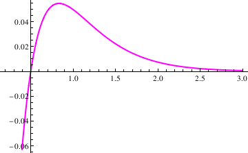
When does the extremum occur?
Where is the extremum?
II. Reduction of Order
1.4.4. Variation of Parameters/Lagrange
I. Case Sensitivity
Suppose the fundamental set of solutions is \( x^3 \) and \( 1/x, \) and the right-hand side function is
\( (x-3)^2 /x , \) so we need to solve the non-homogeneous equation
Then
Now we determine the linear differential operator \( L[y] \) having
\( y_1 (x) \ \mbox{and} \ y_2 (x) \) as solutions of \( L[y]=0. \)
y2[x_] = 1/x
w[x_] = Wronskian[{y1[x], y2[x]}, x]
basis = {x^3, 1/x}
W[x_] = Table[D[basis, {x, i}], {i, 0, 1}]// Flatten
1/4 (-((9 x^2)/2) + 2 x^3 - x^4/4)}
1.4.5. Method of Undetermined Coefficients
L[x_, y_] = y'''[x] - 2 y''[x] - 5 y'[x] + 6 y[x]
rhs = x^3
L[x,y] == rhs
assume[x_] = a0 + a1*x + a2*x^2 + a3*x^3
result = Collect[L[x, assume], x]
eqns = CoefficientList[result, x] == CoefficientList[rhs, x]
yp[x_] = assume[x] /. Solve[eqns][[1]]
1.4.6. Operator Method
I. Case Sensitivity
1.4.7. Numerical Solutions of Second Order ODEs
Example 1.4.3:
Rayleigh's equation is a non-linear equation
\[ x'' + \mu \left( x^2 -1\right) x +x =0 , \]
that arises in the study of the motion of a violin string. We plot three solutions subject to three different initial conditions:
x'[0] == 0}, x[t], {t, 0, 15}]
Plot[Evaluate[x[t] /. {numsol, numsol2, numsol3}], {t, 0, 15},
PlotStyle -> {GrayLevel[0.1], Dashed, Thick}]
To identify each graph, it is helpful to use PlotLegend option:
PlotLegends -> Automatic]
PlotLegends -> {"IC: x(0)=1, x'(0)=0", "IC: x(0)=0.1, x'(0)=0", "IC: x(0)=0, x'(0)=2"}]
I. Pendulum Equation
There seems no doubt that the first person who investigated and established the mathematical theory and properties of the pendulum was
Christiaan Huygens (this spelling of his name is taken from the title of his 1658 book Horologium Oscillatorium), the Dutch
philosopher. The main point of Huygens discovery was that the curve in which a bob hang by a string of insensible weight must move in order to be isochronous in its vibrations, is not a circle, but a cycloid.
For a point pendulum supported by massless, inextensible cord of length \( \ell , \) the equation of motion for oscillations in a vacuum is
The resistance of the air acts on both the pendulum ball and the pendulum wire. It causes the amplitude to decrease with time and increases the period of oscillation slightly. The drag force is proportional to the velocity for values of the Reynolds number of the order 1 or less. For values of the Reynolds number of order \( 10^3 \) to \( 10^5 , \) the force is proportional to the square of the velocity. The maximum Reynolds number based on diameter for the ball is 1100, where the quadratic force law should apply, while the maximum value based on diameter of wire is about 6, where the linear force law should prevail.
Since the damping force is neither linear nor quadratic, but rather a combination of the two, it makes sense to establish a damping function which contains both effects simultaneously. Therefore, the pendulum equation becomes
where \( \alpha = \kappa /(2m) ,\quad \epsilon = c\ell /m, \quad \omega_0 = \left( g/\ell \right)^{1/2} ,\) and \( \mbox{sign}(x) = \begin{cases} 1, & \ x>0, \\ -1, & \ x<0. \end{cases} \)
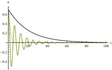
In order to find out the relationship between the angle of the pendulum and time t, a good way is to plot \[Theta] against t.In order to make the plot, first solve the differential equation with the command NDSolve.
This can be done by assigning constant values to \[Alpha],
\[Epsilon], and \[Omega] when using the NDSolve command, get three
different functions in respect to three different \[Alpha] values,
and use the Plot command to plot the three functions in one graph
numsol1 =
NDSolve[{y''[x] == -10*2*y'[x] - Sin[y[x]], y[0] == 0.7, y'[0] == 0},
y[x], {x, 0, 1000}]
numsol2 =
NDSolve[{y''[x] == -1*2*y'[x] - Sin[y[x]], y[0] == 0.7, y'[0] == 0},
y[x], {x, 0, 1000}]
numsol3 =
NDSolve[{y''[x] == -0.1*2*y'[x] - Sin[y[x]], y[0] == 0.7,
y'[0] == 0}, y[x], {x, 0, 1000}]
Plot[Evaluate[y[x] /. {numsol1, numsol2, numsol3}], {x, 0, 100},
PlotRange -> All, PlotStyle -> {GrayLevel[0.1], Dashed, Thick},
AxesLabel -> {"t", "\[Theta]"},
PlotLegends -> {"\[Alpha]=10", "\[Alpha]=1", "\[Alpha]=0.1"}]
Another method is to set up a function that takes \[Theta]0,
\[Omega]0,\[Alpha], \[Epsilon] and tmax as input and out put a function of \[Theta].
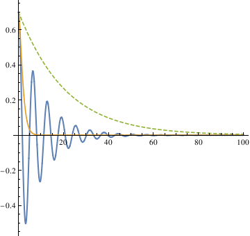
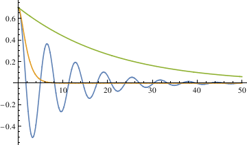
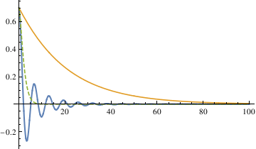
The three different methods all get the same result, from which we can see that the largest damping coefficient does not stop the pendulum the fastest. So the qualitative difference among the three diffrent coefficients is that when \[Alpha] is 0.1, the pendulum oscilates (cross 0). In other cases, the pendulum doesn' t oscilate (doesn' t cross 0).
The critical dammping value is the damping coefficient that stop the \ pendulum the fastest.
In order to find out the critical damping value of alpha, first we \ need to define the meaning of stop, because the pendulum will end up \ always be in very small oscilation.
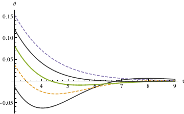
The first method defined - 0.035 < \[Theta] < 0.035 as stop. By plotting different functions of \[Theta] with different alpha \ values (0.6, 0.7, 0.8, 0.9, 1.0) in one graph, you can see that \[Alpha] = 0.7 starts to be in the range [-0.035, 0.035] the fastest.
NDSolve[{y''[x] == -0.6*2*y'[x] - Sin[y[x]], y[0] == 0.7, y'[0] == 0}, y[x], {x, 0, 1000}]
numsolb1 =
NDSolve[{y''[x] == -0.7*2*y'[x] - Sin[y[x]], y[0] == 0.7, y'[0] == 0}, y[x], {x, 0, 1000}]
numsolc1 =
NDSolve[{y''[x] == -0.8*2*y'[x] - Sin[y[x]], y[0] == 0.7, y'[0] == 0}, y[x], {x, 0, 1000}]
numsold1 =
NDSolve[{y''[x] == -0.9*2*y'[x] - Sin[y[x]], y[0] == 0.7, y'[0] == 0}, y[x], {x, 0, 1000}]
numsolf1 =
NDSolve[{y''[x] == -1.0*2*y'[x] - Sin[y[x]], y[0] == 0.7, y'[0] == 0}, y[x], {x, 0, 1000}]
NDSolve[{y''[x] == -0.74*2*y'[x] - Sin[y[x]], y[0] == 0.7, y'[0] == 0}, y[x], {x, 0, 1000}]
numsolb =
NDSolve[{y''[x] == -0.73*2*y'[x] - Sin[y[x]], y[0] == 0.7, y'[0] == 0}, y[x], {x, 0, 1000}]
numsolc =
NDSolve[{y''[x] == -0.72*2*y'[x] - Sin[y[x]], y[0] == 0.7, y'[0] == 0}, y[x], {x, 0, 1000}]
numsold =
NDSolve[{y''[x] == -0.71*2*y'[x] - Sin[y[x]], y[0] == 0.7, y'[0] == 0}, y[x], {x, 0, 1000}]
numsolf =
NDSolve[{y''[x] == -0.70*2*y'[x] - Sin[y[x]], y[0] == 0.7, y'[0] == 0}, y[x], {x, 0, 1000}]
numsolg =
NDSolve[{y''[x] == -0.69*2*y'[x] - Sin[y[x]], y[0] == 0.7, y'[0] == 0}, y[x], {x, 0, 1000}]
numsolh =
NDSolve[{y''[x] == -0.68*2*y'[x] - Sin[y[x]], y[0] == 0.7, y'[0] == 0}, y[x], {x, 0, 1000}]
numsoli =
NDSolve[{y''[x] == -0.67*2*y'[x] - Sin[y[x]], y[0] == 0.7, y'[0] == 0}, y[x], {x, 0, 1000}]
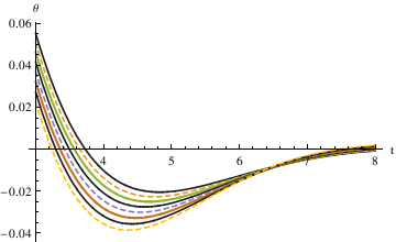
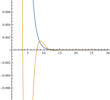
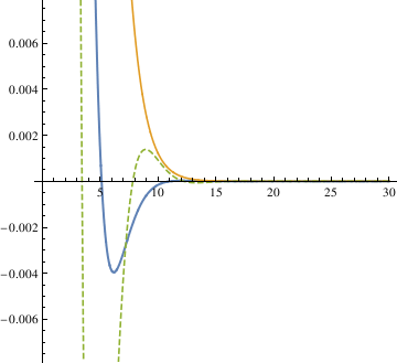
When \[Alpha] = 0.85, the pendulum settles in the range faster than when \[Alpha] = 1. So the critical value may be smaller than 0.85. Try the mid value of 0.85 and 0.7. Finally, the answer got from this method is 0.81.
The third method defines stop as not passing 0 in the time span 0 < t \ < 500, uses a function "piano" to check if the pendulum oscilates.
\[CapitalOmega]0 = 1;
listofsolutions = {};
listofvaluesfor\[Alpha] = Range[0, 2, .0005];
pendulumeq = \[Theta]''[t] + 2*\[Alpha]*\[Theta]'[t] + \[CurlyEpsilon]* Sign[\[Theta]'[t]]*((\[Theta]'[t])^2) + (\[CapitalOmega]0^2)* Sin[\[Theta][t]] == 0;
Catch[If[FindMinValue[ evaluatedlistofsolutions[[key]], {t, 0, 500}] > 0, Throw[key], Throw[906]]];
Module[{\[Theta]}, \[Theta] /. First[ NDSolve[{ \[Theta]''[t] == -Sin[\[Theta][t]] - 2 \[Alpha] \[Theta]'[ t] - \[Epsilon] Sign[\[Theta]'[t]] (\[Theta]'[t])^2, \[Theta][0] == \[Theta]0, \[Theta]'[0] == \[Omega]0}, \[Theta], {t, 0, tmax}] ]]
II. Spring Equation
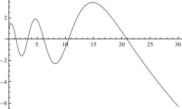
Consider the following spring equation with aging:
We solve it and plot in the following sequence of steps.
x, t] // InputForm
{{x -> Function[{t}, (BesselJ[0, 16*Sqrt[E^(-t/4)]]*
BesselY[0, 16] - BesselJ[0, 16]*BesselY[0,
16*Sqrt[E^(-t/4)]] + BesselJ[1, 16]*
BesselY[0, 16*Sqrt[E^(-t/4)]] -
BesselJ[0, 16*Sqrt[E^(-t/4)]]*BesselY[1, 16])/
(BesselJ[1, 16]*BesselY[0, 16] - BesselJ[0, 16]*
BesselY[1, 16])]}}
x, t]) // InputForm
f[t_] = x[t] /. sol[[1]]
f[0.5]
Another way to remove curly brackets:
(BesselJ[0, 16 Sqrt[E^(-t/4)]] BesselY[0, 16] -
BesselJ[0, 16] BesselY[0, 16 Sqrt[E^(-t/4)]] +
BesselJ[1, 16] BesselY[0, 16 Sqrt[E^(-t/4)]] -
BesselJ[0, 16 Sqrt[E^(-t/4)]] BesselY[1, 16])/(BesselJ[1,
16] BesselY[0, 16] - BesselJ[0, 16] BesselY[1, 16])
1.4.9. Applications
We present some applications of differential equations of order greater than one.
Example 4.9.1: Flow Problems
A 500 liter container initially contains 10 kg of salt. A brine mixture of 100 gramms
of salt per liter is entering the container at 6 liter per minute. The well-mixed contents
are being discharged from the tank at the rate of 6 liters per minute.
Express the amount of salt in the container as a function of time.
Salt is coming at the rate: 6*(0.1)=0.6 kg/min
d yin /dt =0.6 ; d yout/dt = 6x/500
dx/dt = 0.6 -6x/500 ; x(0)=10
Suppose that the rate of discharge is reduced to 5 liters per minute.
SolRule[t_] = Apart[x[t] /. First[%]]
Together[SolRule'[t] == Together[6/10 - 5*SolRule[t]/(500 + t)]]
SolRule[0]
Out[4]= True
Out[5]= 10
Example 4.9.2: Pure oscillations give the solutions of the following differential equation subject to the given initial conditions (displacement is 1, but velocity is zero):
soln = DSolve[{x''[t] + 25 x[t] == 0, x[0] == 1, x'[0] == 0}, x[t], t]
Plot[x[t] /. soln, {t, -1, 2.5}]
s[t_] = x[t]/.soln[[1]]
Plot[s[t],{t,0,3},AxesLabel->{"t","Displacement"}]
Example 4.9.3: Consider the initial value problem
s1[t_] = x[t] /. soln[[1]]
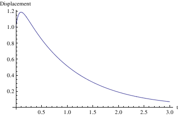
When does the maximum excursion occur?
Example 4.9.4: Now we turn to a differential equation whose characteristic polynomial has a double root:
s2[t_] = x[t] /. soln[[1]]
Plot[s2[t], {t, 0.2, 3}, PlotStyle->{Thick,Magenta}]
Out[12]= E^(-3 t) (-1 + 2 t)
Out[13]=

When does the extremum occur?
Example 4.9.5: We consider another initial value problem
x'[0] == 5}, x[t], t]
soln = DSolve[{x''[t] + 2 x'[t] + 37 x[t] == 0, x[0] == -1, x'[0] == 5}, x[t], t]
s3[t_] = x[t] /. soln[[1]]
Plot[s3[t], {t, 0, 3}, PlotRange -> {-1, 1}]
Out[20]= -(1/3) E^-t (3 Cos[6 t] - 2 Sin[6 t])
Out[21]=
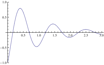
Now we define the amplitude of these oscillations:
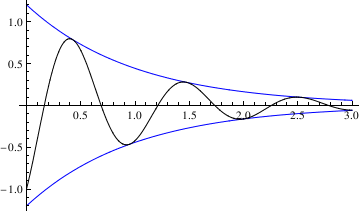
Example 4.9.6: Forced oscillations are modelled by the following nonhomogeneous equation:
1/712 E^(-5 t) (-392 Cos[4 t] - 445 E^(5 t) Cos[4 t] +
125 E^(5 t) Cos[4 t] Cos[8 t] + 200 Sin[4 t] -
200 E^(5 t) Cos[8 t] Sin[4 t] + 200 E^(5 t) Cos[4 t] Sin[8 t] +
125 E^(5 t) Sin[4 t] Sin[8 t])}}
We extract the transient solution and the steady-state solution. First, we define the solution function:
40 E^(5 t) Cos[8 t] Sin[4 t] + 40 E^(5 t) Cos[4 t] Sin[8 t] + 25 E^(5 t) Sin[4 t] Sin[8 t])
40 Cos[8 t] Sin[4 t] - 40 Cos[4 t] Sin[8 t] - 25 Sin[4 t] Sin[8 t])}}
40 Cos[8 t] Sin[4 t] - 40 Cos[4 t] Sin[8 t] - 25 Sin[4 t] Sin[8 t])
Now we consider a similar problem but with another input function:
L[t_,x_] = x''[t] + 10 x'[t] + 41 x[t];
solnRule = DSolve[{L[t, x] == 8 *Exp[-5*t] Cos[2 t], x[0] == -1, x'[0] == 5}, x[t], t]
1/6 E^(-5 t) (-13 Cos[4 t] + 6 Cos[t]^2 Cos[4 t] +
Cos[4 t] Cos[6 t] + 3 Sin[2 t] Sin[4 t] + Sin[4 t] Sin[6 t])}}
Cos[4 t] Cos[6 t] + 3 Sin[2 t] Sin[4 t] + Sin[4 t] Sin[6 t])
E^(-5 t) C[2] Cos[4 t] + E^(-5 t) C[1] Sin[4 t] +
1/6 E^(-5 t) (6 Cos[t]^2 Cos[4 t] + Cos[4 t] Cos[6 t] +
3 Sin[2 t] Sin[4 t] + Sin[4 t] Sin[6 t])}}
1/6 E^(-5 t) (6 Cos[t]^2 Cos[4 t] + Cos[4 t] Cos[6 t] +
3 Sin[2 t] Sin[4 t] + Sin[4 t] Sin[6 t])
and the transient solution becomes
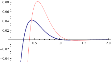
We also plot two solutions
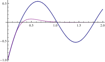
Transient solutions could be plotted ina similar way.
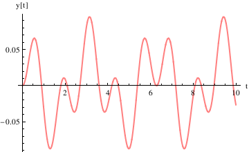
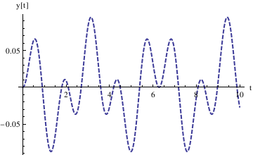
Example 4.9.7: Undamped Spring with External Forcing.
Enter the coefficients and the differential equation:
ode = y''[t] + k^2*y[t] == F0*Cos[omega*t];
1/210 (-10 Cos[5 t] + 7 Cos[3 t] Cos[5 t] + 3 Cos[5 t] Cos[7 t] +
7 Sin[3 t] Sin[5 t] + 3 Sin[5 t] Sin[7 t])}}
7 Sin[3 t] Sin[5 t] + 3 Sin[5 t] Sin[7 t])
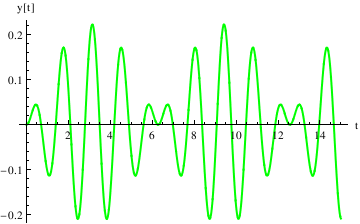
Example 4.9.8: Beats
We reconsider Example 1.4.7 for periodic input, when resonance is observed.
Enter the coefficients and the differential equation.
ode = y''[t] + k^2*y[t] == F0*Cos[omega*t];
1/90 (-10 Cos[5 t] + 9 Cos[t] Cos[5 t] + Cos[5 t] Cos[9 t] +
9 Sin[t] Sin[5 t] + Sin[5 t] Sin[9 t])}}
9 Sin[t] Sin[5 t] + Sin[5 t] Sin[9 t])
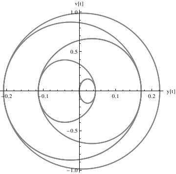
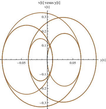
Define the derivative function as v[t], and plot the trajectory in the phase plane:
4 Cos[9 t] Sin[5 t] - 4 Cos[5 t] Sin[9 t])
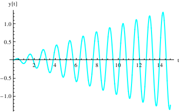
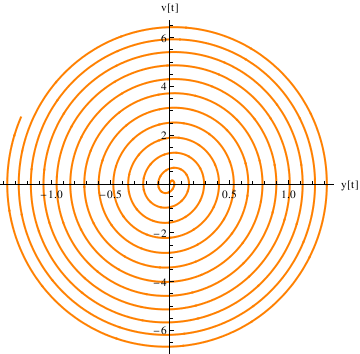
Example 4.9.9: Resonance
We repeat the commands (after quitting the kernel) here for defining the coefficients and the differential equation---now with \[omega] very close to k:
ode = y''[t] + k^2*y[t] == F0*Cos[omega*t];
DSolve[{ode, y[0] == 0, y'[0] == 0}, y[t], t]
0.010101 Cos[5. t] Cos[9.9 t] + 1. Sin[0.1 t] Sin[5. t] +
0.010101 Sin[5. t] Sin[9.9 t] }}
1.0101 Cos[4.9 t] Sin[5. t]^2
4.94949 Sin[4.9 t] Sin[5. t]^2
ode = y''[t] + k^2*y[t] == F0*Cos[omega*t];
DSolve[{ode, y[0] == 0, y'[0] == 0}, y[t], t]
y[t_] = y[t] /. %[[1]]
1/210 (-10 Cos[5 t] + 7 Cos[3 t] Cos[5 t] + 3 Cos[5 t] Cos[7 t] +
7 Sin[3 t] Sin[5 t] + 3 Sin[5 t] Sin[7 t])}}
Out[4]= 1/210 (-10 Cos[5 t] + 7 Cos[3 t] Cos[5 t] + 3 Cos[5 t] Cos[7 t] +
7 Sin[3 t] Sin[5 t] + 3 Sin[5 t] Sin[7 t])
1.4.8. References
Martha L. Abell, James P. Braselton
Differential Equations With Mathematica,
Academic Press, 2004
ISBN 0120415623, 978012041562
Alfred Gray, Mike Mezzino, and Mark Pinsky
Introduction to Ordinary Differential Equations with Mathematica: An Integrated Multimedia Approach
Springer
ISBN-10: 0387944818 | ISBN-13: 978-0387944814
Brian R. Hunt, Ronald L. Lipsman, John E. Osborn, Donald A. Outing, Jonathan Rosenberg
Differential Equations with Mathematica, 3rd Edition
ISBN: 978-0-471-77316-0
Clay C. Ross
Differential Equations
An introduction with Mathematica
Springer-Verlag, 1995
ISBN: 0-387-94301-3


