Let us consider a stiff massless rod of length ℓ and mass
m, whose suspension point
A oscillates vertically according to
yA = 𝑎sin(ω
t)
rod = Graphics[{LightGray,
Polygon[{{-0.05, 1.0}, {0.0, 1.01}, {0.25, 0.05}, {0.2, 0.03}}]}];
ball = Graphics[{Orange, Disk[{0.27, -0.1}, 0.15]}];
ball2 = Graphics[{Black, Disk[{0.08, 0.6}, 0.02]}];
ball3 = Graphics[{Black, Disk[{-0.02, 1.0}, 0.01]}];
ar = Graphics[{Black, Thickness[0.01], Arrowheads[0.08],
Arrow[{{-0.02, 1.0}, {-0.02, 0.7}}]}];
ar2 = Graphics[{Black, Thickness[0.01], Arrowheads[0.08],
Arrow[{{-0.2, 0.5}, {0.3, 0.5}}]}];
ar3 = Graphics[{Black, Thickness[0.01], Arrowheads[0.08],
Arrow[{{-0.16, 0.5}, {-0.16, 1.0}}]}];
tl = Graphics[{Black,
Text[Style["\[ScriptL]", 18, FontFamily -> "Mathematica1"], {0.27,
0.1}]}];
tx = Graphics[{Black, Text[Style["x", 18], {0.28, 0.45}]}];
tcm = Graphics[{Black, Text[Style["CM", 18], {0.17, 0.6}]}];
t2 = Graphics[{Black, Text[Style["\[Theta]", 18], {0.05, 0.4}]}];
line = Graphics[{Black, Dashed, Thick,
Line[{{-0.02, 1.1}, {-0.02, 0}}]}];
t3 = Graphics[{Black,
Text[Style[Subscript[a, A], 18], {-0.08, 0.72}]}];
t4 = Graphics[{Black,
Text[Style["a sin(\[Omega]t)", 18], {-0.15, 1.05}]}];
t5 = Graphics[{Black, Text[Style["A", 18], {0.02, 1.0}]}];
Show[rod, ar, ar2, ar3, tl, tx, ball2, ball3, tcm, t2, t3, line, t4,
t5]
Pendulum with support moving vertically.
Then the equation of motion becomes
\[
I_A \ddot{\theta} + mg\,\frac{\ell}{2} \,\sin\theta = \frac{m\ell}{2}\, a\,\omega^2 \sin (\omega t)\,\sin\theta .
\]
Example 1:
Consider a mathematical pendulum whose support moves periodically in a vertical direction (Fig.1(a)). The governing differential equation is
\[
\frac{{\text d}^2 x}{{\text d} t^2} + \left( \frac{g}{\ell} - \frac{A \omega^2}{\ell}\,\cos (\omega t) \right) \sin x (t) = 0 ,
\]
where
x is the generalized coordinate being the angle of deflection,
g is the acceleration of gravity, ℓ is the pendulum’s length,while the vertical motion of the support is
Acos(ωt). However, by introducing τ = ω
t, one can obtain
\[
\frac{{\text d}^2 x}{{\text d} \tau^2} + \left( \frac{g}{\ell \omega^2} - \frac{A}{\ell}\,\cos (\tau ) \right) \sin x (\tau ) = 0 ,
\]

|
|
This equation includes, besides the torque −mgℓ sin(x) of the gravitational force mg, the instantaneous torque of the force of inertial, which depends explicitly on time t.
rec = Graphics[{Pink, Rectangle[{-0.5, -1}, {0.5, 1}]}];
rod = Graphics[{Thickness[0.05], Blue, Line[{{0, 0}, {1, -3}}]}];
line = Graphics[{Dashed, Line[{{0, 0}, {0, -2}}]}];
mass = Graphics[{Gray, Disk[{1, -3}, 0.15]}];
ell = Graphics[{Text[
Style[ToExpression["\ell", TeXForm],
FontSize -> 20], {0.7, -1.5}]}];
m = Graphics[Text[Style["m", FontSize -> 20], {1.3, -3}]];
line2 = Graphics[{Dashed, Line[{{0, 0}, {1, 0}}]}];
a = Graphics[{Thickness[0.01], Arrowheads[0.1],
Arrow[{{0.8, 0}, {0.8, 1.0}}]}];
txt = Graphics[
Text[Style["A cos(\[Omega]t)", FontSize -> 20], {1.3, 0.6}]];
x = Graphics[Text[Style["x", FontSize -> 20], {0.2, -1.6}]];
Show[rec, rod, m, line, line2, ell, mass, a, txt, x]
|
|
Periodicly excited pivot
|
|
Mathematica code
|
Upon including the frictional torque, which is assumed in this model to be proportional to the momentary value of the angular velocity, with the damping constant γ, we get
\[
\frac{{\text d}^2 x}{{\text d} t^2} + \gamma\,\frac{{\text d} x}{{\text d} t} + \left( \frac{g}{\ell} - \frac{A \omega^2}{\ell}\,\cos (\omega t) \right) \sin x (t) = 0 ,
\]
■
Example 2:
Let us consider a solid massless rod of length ℓ and mass
m2 suspended on a spring damper system with mass
m1 and stiffness
k and damping factor
d. Mass
m1 can move only in the depicted y direction and pendulum only in the
x-y plane. The mechanical system has two degrees of freedom because the slab can move only vertically and the pendulum position is identified by angle θ.
string = Graphics[{Black, Thick,
Line[{{0.0, 0.0}, {0.0, 0.2}, {-0.25, 0.4}, {0.25, 0.6}, {-0.25,
0.8}, {0.25, 1}, {-0.25, 1.2}, {0.25, 1.4}, {0, 1.6}, {0, 2}}]}];
rod = Graphics[{Gray, Rectangle[{0.55, 0.65}, {1.05, 0.85}]}];
rod2 = Graphics[{Orange, Rectangle[{-0.4, 2.0}, {1.1, 2.25}]}];
rod3 = Graphics[{Gray, Rectangle[{-0.4, 0.0}, {1.1, -0.1}]}];
rod0 = Graphics[{Blue, Thickness[0.01],
Line[{{0.45, 2.0}, {1.5, 0.5}}]}];
ball = Graphics[{Orange, Disk[{1.5, 0.5}, 0.15]}];
damp = Graphics[{Black, Thickness[0.01],
Line[{{0.8, 0.0}, {0.8, 0.6}}]}];
damp2 = Graphics[{Black, Thick,
Line[{{0.5, 0.9}, {0.5, 0.6}, {1.1, 0.6}, {1.1, 0.9}}]}];
line = Graphics[{Black, Dashed, Thick,
Line[{{0.4, 2.1}, {0.4, 2.5}}]}];
line2 = Graphics[{Black, Dashed, Thick,
Line[{{0.4, 2.1}, {0.1, 2.5}}]}];
line3 = Graphics[{Black, Dashed, Thick,
Line[{{-0.4, -0.05}, {-0.8, -0.05}}]}];
line4 = Graphics[{Black, Dashed, Thick,
Line[{{-0.4, 2.1}, {-0.8, 2.1}}]}];
ar = Graphics[{Black, Thickness[0.005], Arrowheads[0.08],
Arrow[{{-0.7, -0.05}, {-0.7, 2.1}}]}];
ty = Graphics[{Black, Text[Style["y(t)", 18], {-0.5, 1.0}]}];
tl = Graphics[{Black,
Text[Style["\[ScriptL]", 18, FontFamily -> "Mathematica1"], {1.1,
1.3}]}];
t2 = Graphics[{Black, Text[Style["\[Theta]", 18], {0.3, 2.4}]}];
tm1 = Graphics[{Black,
Text[Style[Subscript[m, 1], 18], {1.35, 2.1}]}];
tm2 = Graphics[{Black,
Text[Style[Subscript[m, 2], 18], {1.5, 0.25}]}];
Show[damp, damp2, damp3, string, ball, rod, rod0, rod2, rod3, line,
line2, line3, line4, ar, tl, t2, ty, tm1, tm2]
Pendulum attached to moving slab.
Governing equations are derived using the Lagrange formalism. Considering the frame of reference at the origin placed on the slab and defining in Cartesian coordinates two vectors ry and rθ
\[
{\bf r}_y = \begin{pmatrix} 0 \\ y(t)
\end{pmatrix} , \qquad {\bf r}_{\theta} = \begin{pmatrix} \ell\,\sin\theta \\ y(t) - \ell\,\cos\theta
\end{pmatrix} .
\tag{2.1}
\]
The kinetic energy is the sum of corresponding energies for the slab
\[
\mbox{K}_y = \frac{1}{2}\, m_1 \dot{y}^2 ,
\]
and for the pendulum
\[
\mbox{K}_{\theta} = \frac{1}{2}\, m_2 \left[ \dot{\theta}^2 \ell^2 \cos^2 + \left( \dot{y}+\ell\,\dot{\theta}\,\sin\theta \right)^2 \theta \right]
\]
Both elements of the system (slab and pendulum) contribute to the potential energy
\[
\Pi_y = m_1 g\,y + \frac{k}{2}\,y^2
\]
and
\[
\Pi_{\theta} = m_2 g\left( y - \ell\,\cos\theta \right) .
\]
Then the Laprangian for the system becomes
\[
{\cal L} = \mbox{K}_y +\mbox{K}_{\theta} - \Pi_y - \Pi_{\theta}
\]
We need to take into account
the viscous friction for both elements
\[
T_y = d\,\dot{y} \qquad\mbox{and} \qquad T_{\theta} = D\,\dot{\theta} .
\]
If there exists an oscillated driving force, we model it as
\[
F_0 = - \left( m_1 + m_2 \right) \frac{{\text d}^2}{{\text d} t^2} \left( A\,\cos \omega t \right) = \left( m_1 + m_2 \right) A\omega^2 \cos\omega t .
\]
Application of the Lagrange formalism
\[
\frac{\partial {\cal L}}{\partial q_i} - \frac{\text d}{{\text d}t} \,\frac{\partial {\cal L}}{\partial \dot{q}_i} + \sum_{k=1}^2 \lambda_k \frac{\partial f_i}{\partial q_k} = 0
\]
to the system with two degrees of freedom yields the system of non-linear differential equations
\begin{align*}
\left( m_1 + m_2 \right) \ddot{y} + g \left( m_1 + m_2 \right) + ky + \ell m_2 \left( \dot{\theta}^2 \cos\theta + \ddot{\theta} \sin\theta \right) &= -d\,\dot{y} + F_0 ,
\\
m_2 \ell^2 \ddot{\theta} + g\ell m_2 \sin]theta + \ell m_2 \ddot{y} \sin\theta &= -D\dot{\theta} .
\end{align*}
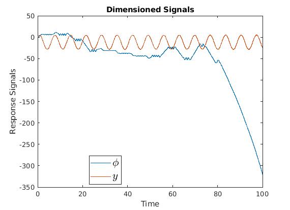
syms y(t) phi(t)
d1y = diff(y,1);
d2y = diff(y,2);
d1phi = diff(phi,1);
d2phi = diff(phi,2);

%Parameter Values
m1 = 1;
m2 = 2;
l = 0.5;
g = 9.81;
k = 2.5;
d = 0; % No Damping
F0 = 0; % No external Force
D = 0; % No Damping

%Equation ODE Solver
eq1 = (m1+m2)*d2y + g*(m1+m2)+ k*y + l*m2*(d1phi^2*cos(phi) + d2phi*sin(phi))+d*y-F0 == 0;
eq2 = m2*l^2*d2phi + g*l*m2*sin(phi) + l*m2*d2y*sin(phi)+ D * d1phi == 0;
[F, S] = odeToVectorField(eq1, eq2);
odeFun = matlabFunction(F, 'Vars', {t, 'Y'});
[t, x] = ode45(odeFun, [0 100], [0.5; 0.5; pi/6; 10]);

%% Plot 1 - Dimensioned Signals
figure(1)
plot(t, x(:,[1,3]));
legend({'$\phi$', '$y$'}, ...
    'FontSize', 16, ...
    'Interpreter', 'latex', ...
    'Location', 'best');
title('Dimensioned Signals')
xlabel('Time')
ylabel('Response Signals')
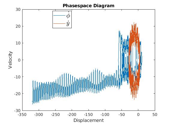
%% Plot 2 - Phasespace Diagram
figure(2)
plot(x(:,1),x(:,2),x(:,3),x(:,4));
legend({'$\dot{\phi}$', '$\dot{y}$'}, ...
    'FontSize', 16, ...
    'Interpreter', 'latex', ...
    'Location', 'best');
title('Phasespace Diagram')
xlabel('Displacement')
ylabel('Velocity')
|
|
|
|
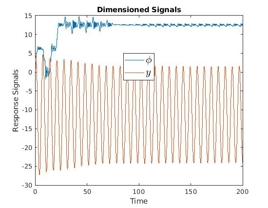
syms y(t) phi(t)
d1y = diff(y,1);
d2y = diff(y,2);
d1phi = diff(phi,1);
d2phi = diff(phi,2);

%Parameter Values
m1 = 1;
m2 = 2;
l = 0.5;
g = 9.81;
k = 2.5;
d = 0.1; % Damping exists
F0 = 0.05;
D = 0.2; % Damping exists

%Equation ODE Solver
eq1 = (m1+m2)*d2y + g*(m1+m2)+ k*y + l*m2*(d1phi^2*cos(phi) + d2phi*sin(phi))+d*y-F0 == 0;
eq2 = m2*l^2*d2phi + g*l*m2*sin(phi) + l*m2*d2y*sin(phi)+ D * d1phi == 0;
[F, S] = odeToVectorField(eq1, eq2);
odeFun = matlabFunction(F, 'Vars', {t, 'Y'});
[t, x] = ode45(odeFun, [0 200], [0.5; 0.1; pi/6; 10]);

%% Plot 1 - Dimensioned Signals
figure(1)
plot(t, x(:,[1,3]));
legend({'$\phi$', '$y$'}, ...
    'FontSize', 16, ...
    'Interpreter', 'latex', ...
    'Location', 'best');
title('Dimensioned Signals')
xlabel('Time')
ylabel('Response Signals')
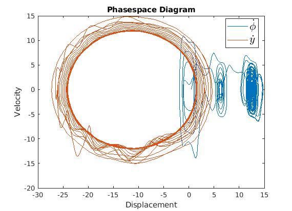
%% Plot 2 - Phasespace Diagram
figure(2)
plot(x(:,1),x(:,2),x(:,3),x(:,4));
legend({'$\dot{\phi}$', '$\dot{y}$'}, ...
    'FontSize', 16, ...
    'Interpreter', 'latex', ...
    'Location', 'best');
title('Phasespace Diagram')
xlabel('Displacement')
ylabel('Velocity')
|
|
|
|
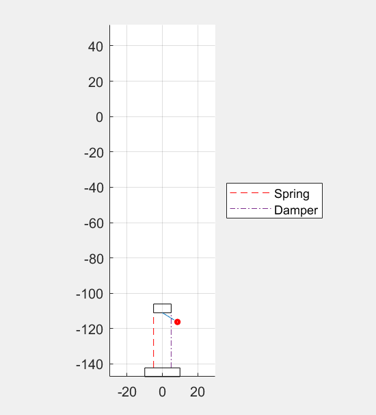
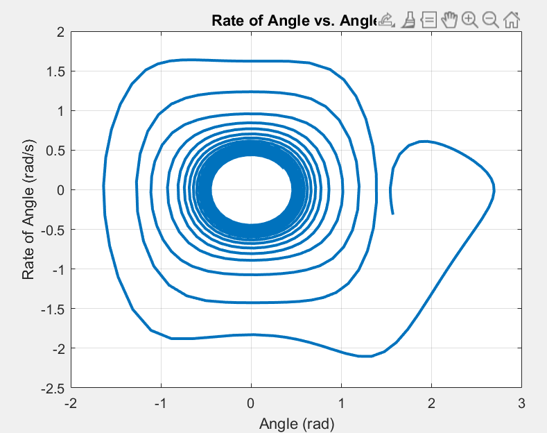
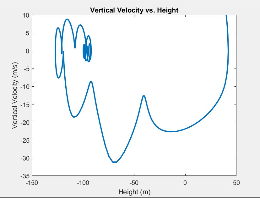
We present matlab for another choice of coefficients
 syms m1 m2 k d D l y(t) theta(t) g F0 T Y

eq1 = diff(y,1) == (F0-((m1+m2)*diff(y,2) + g*(m1+m2) + k*y + l*m2*(((diff(theta,1)^2)*cos(theta))+(diff(theta,2)*sin(theta)))))/d;
eq2 = diff(theta,1) == -(m2*(l^2)*diff(theta,2) + g*l*m2*sin(theta) + l*m2*diff(y,2)*sin(theta))/D;

[V,S] = odeToVectorField(eq1,eq2);
fxn = matlabFunction(V,'Vars',{T,Y,m1,m2,k,d,D,l,g,F0});

m1 = 2; m2 = 3; k = 0.5; d = 1.5; D = 0.1; l = 10;
g = 9.81; F0 = 0;

times = [0,100];
ic = [0.5*pi,-0.1*pi,40,10]; %[theta, Dtheta, y, Dy]

[t,sols] = ode45(@(T,Y)fxn(T,Y,m1,m2,k,d,D,l,g,F0),times,ic);

angle = sols(:,1); Dangle = sols(:,2); height = sols(:,3); Dheight = sols(:,4);

figure
plot(t,angle,'LineWidth',2)
grid
xlabel('Time (s)')
ylabel('Angle (rad)')
title('Angle vs. Time')

figure
plot(t,height,'LineWidth',2)
grid
xlabel('Time (s)')
ylabel('Height (m)')
title('Height vs. Time')

figure
plot(angle,Dangle,'LineWidth',2)
grid
xlabel('Angle (rad)')
ylabel('Rate of Angle (rad/s)')
title('Rate of Angle vs. Angle')

figure
plot(height,Dheight,'LineWidth',2)
hold on
xlabel('Height (m)')
ylabel('Vertical Velocity (m/s)')
title('Vertical Velocity vs. Height')

%%%%%%%%%%%%%%%%%%%%%%%%%%%%%%%%%%%%%%%%%%%%%%% ANIMATE ??????????????

figure
axis equal; grid on; axis([-30 30 min(sols(:,3))-20 max(sols(:,3))+10]);
set(legend,'Location','eastoutside');

for i = 1:length(t)
    O = [0 sols(i,3)];
    P = [O(1)+l*sin(sols(i,1)) O(2)-l*cos(sols(i,1))];
    rect_O = rectangle("Position",[O(1)-5 O(2) 10 5]);
    spring = line([-5 -5],[min(sols(:,3))-15 O(2)],'Color','red','LineStyle','--','DisplayName','Spring');
    damper = line([5 5],[min(sols(:,3))-15 O(2)],'Color','#7E2F8E','LineStyle','-.','DisplayName','Damper');
    rod = line([O(1) P(1)], [O(2) P(2)],'HandleVisibility','off');
    ball = viscircles(P,1);
    base = rectangle('Position',[-10 min(sols(:,3))-20 20 5]);
    pause(0.001)
    if i
|
|
|
■
Let us consider a pendulumof length ℓ and mass
m whose suspension point
A oscilates horisontally according to
xA = 𝑎 sin ω
t. Then its motion is modeled by
\[
I_A \ddot{\theta} + mg\,\frac{\ell}{2}\,\sin\theta = mg\,\frac{\ell}{2}\,a \omega^2 \sin\omega t\,\cos\theta .
\]
rod = Graphics[{LightGray,
Polygon[{{-0.05, 1.0}, {0.0, 1.01}, {0.25, 0.05}, {0.2,
0.03}}]}];
ball2 = Graphics[{Black, Disk[{0.08, 0.6}, 0.02]}];
ball3 = Graphics[{Black, Disk[{-0.02, 1.0}, 0.01]}];
ar = Graphics[{Black, Thickness[0.01], Arrowheads[0.08],
Arrow[{{-0.02, 1.0}, {-0.22, 1.0}}]}];
tl = Graphics[{Black,
Text[Style["\[ScriptL]", 18, FontFamily -> "Mathematica1"], {0.27,
0.1}]}];
tx = Graphics[{Black, Text[Style["x", 18], {0.27, 1.04}]}];
tcm = Graphics[{Black, Text[Style["CM", 18], {0.17, 0.6}]}];
t2 = Graphics[{Black, Text[Style["\[Theta]", 18], {0.05, 0.4}]}];
t3 = Graphics[{Black,
Text[Style[Subscript[a, A], 18], {-0.12, 0.95}]}];
t4 = Graphics[{Black,
Text[Style["a sin(\[Omega]t)", 18], {-0.15, 1.05}]}];
t5 = Graphics[{Black, Text[Style["A", 18], {0.02, 1.05}]}];
ty = Graphics[{Black, Text[Style["y", 18], {-0.27, 1.18}]}];
line = Graphics[{Black, Dashed, Thick,
Line[{{-0.02, 1.1}, {-0.02, 0}}]}];
line2 = Graphics[{Black, Thick, Line[{{-0.35, 1.0}, {0.28, 1.0}}]}];
line3 = Graphics[{Black, Thick, Line[{{-0.3, 0.0}, {-0.3, 1.2}}]}];
Show[rod, ar, tl, tx, ty, ball2, ball3, tcm, t2, t3, line, t4, t5,
line2, line3]
Pendulum with support moving horizontally.
The length of the pendulum is increasing by the stretching of the wire due to the weight of the bob. The effective
spring constant for a wire of rest length \( \ell_0 \) is
\[
k = ES/ \ell_0 ,
\]
where the elastic modulus (Young's modulus) for steel is about
\( E \approx 2.0 \times 10^{11} \)
Pa and
S is the cross-sectional area. With pendulum 3 m long,
the static increase in elongation is about
\( \Delta \ell = 1.6 \) mm, which is clearly not negligible. There is also dynamic
stretching of the wire from the apparent centrifugal and Coriolis forces acting on the bob during motion. We can
evaluate this effect by adapting a spring-pendulum system analysis. We go from rectangular to polar coordinates:
\[
x= \ell \,\sin \theta = z_0 \left( 1 + \xi \right) \sin \theta , \qquad z= z_0 - \ell\,\cos \theta = z_0 \left[ 1 - \left( 1 + \xi \right) \cos \theta \right] , ,
\]
where
\( z_0 = \ell_0 + mg/k \) is the static pendulum length,
\( \ell = z_0 \left( 1 + \xi \right) \) is the dynamic length, ξ is the fractional
string extension, and θ is the deflection angle. The equations of motion for small deflections are
\begin{eqnarray*}
\left( 1 + \xi \right)\ddot{\theta} + 2\dot{\theta}\,\dot{\xi} +
\omega_p^2 \theta &=& 0 , \\
\ddot{\xi} + \omega_s^2 \xi - \dot{\theta} + \frac{1}{2}\,\omega_p^2 \theta^2
&=& 0,
\end{eqnarray*}
where the overdots denote differentiation with respect to time
t,
\( \omega_p^2 = g/z_0 \)
is the square of the pendulum frequency, and
\( \omega_s^2 = k/m \) is the spring
(string) frequency, squared.
To get a feeling for how rigid and massive the pendulum support must be, we model the support as mass M
kept in place by a spring of constant K, as shown in the picture below.
p = Rectangle[{-Pi/6 - 1.2, 2}, {-5, -5}]
a = Graphics[{Gray, p}]
coil = ParametricPlot[{t + 1.2*Sin[3*t],
1.2*Cos[3*t] - 1.2}, {t, -Pi/6 , 5*Pi - Pi/6}, FrameTicks -> None,
PlotStyle -> Black]
line = Graphics[{Thick, Line[{{16.3843645, -1.2}, {20, -1.2}}]}]
r = Graphics[{EdgeForm[{Thick, Blue}], FaceForm[],
Rectangle[{20, -5}, {26, 2}]}]
back = RegionPlot[-5 < x < 28 || -7 < y < -5, {x, -5,
28}, {y, -7, -5}, PlotStyle -> LightOrange]
line2 = Graphics[{Thick, Dashed, Line[{{23, -1}, {23, -14}}]}]
line3 = Graphics[{Thick, Line[{{23, -1}, {29, -11.5}}]}]
disk = Graphics[{Pink, Disk[{29.5, -12}, 1]}]
text = Graphics[Text["\[Theta]" , {25.1, -9.5}]]
Show[a, coil, line, r, back, line2, line3, disk, text]
Pendulum with support moving horizontally.
The natural frequency of the support is
\[
\Omega = \left( K/M \right)^{1/2} .
\]
The coupled equations for the system are
\begin{eqnarray*}
\ddot{\theta} + \omega_0^2 \theta + \ddot{x}/\ell &=& 0 , \\
\left( 1 + m/M \right) \ddot{x} + \left( m/M \right) \ell \,\ddot{\theta} + \Omega^2 x &=& 0,
\end{eqnarray*}
where
x is the displacement of the rigid support. The former equation says that the effect of sway is to
impart an additional angular acceleration
\( - \ddot{x}/\ell \) to the pendulum
for small angles of oscillation (otherwise, we have to use
\( \omega_0^2 \sin \theta \)
instead of
\( \omega_0^2 \theta \) ).
Let us consider a pendulum of length ℓ and mass
m whose suspension point
A moves with a constant angular frequency ω on a vertical circumference of radius
R. In this case, the governing differential equation becomes
\[
I_A \ddot{\theta} + mg\,\frac{\ell}{2}\,\sin\theta = m\,\frac{\ell}{2}\,a\omega^2 \cos \left( \omega t - \theta \right) .
\]
rod = Graphics[{LightGray,
Polygon[{{-0.05, 1.0}, {0.0, 1.01}, {0.25, 0.05}, {0.2,
0.03}}]}];
ball2 = Graphics[{Black, Disk[{0.105, 0.5}, 0.02]}];
ball3 = Graphics[{Black, Disk[{-0.02, 1.0}, 0.01]}];
ar = Graphics[{Black, Thickness[0.01], Arrowheads[0.08],
Arrow[{{-0.02, 1.0}, {-0.138, 0.74}}]}];
line = Graphics[{Black, Dashed, Thick,
Line[{{-0.02, 1.1}, {-0.02, 0}}]}];
line2 = Graphics[{Black, Thick, Line[{{-0.2, 0.6}, {0.3, 0.6}}]}];
line3 = Graphics[{Black, Thick, Line[{{-0.2, 0.0}, {-0.2, 1.2}}]}];
line4 = Graphics[{Black, Thick, Line[{{-0.2, 0.6}, {-0.02, 1.0}}]}];
ty = Graphics[{Black, Text[Style["y", 18], {-0.24, 1.18}]}];
tl = Graphics[{Black,
Text[Style["\[ScriptL]", 18, FontFamily -> "Mathematica1"], {0.27,
0.1}]}];
tx = Graphics[{Black, Text[Style["x", 18], {0.3, 0.65}]}];
tcm = Graphics[{Black, Text[Style["CM", 18], {0.17, 0.55}]}];
t2 = Graphics[{Black, Text[Style["\[Theta]", 18], {0.05, 0.4}]}];
t3 = Graphics[{Black,
Text[Style[Subscript[a, A], 18], {-0.12, 0.95}]}];
t4 = Graphics[{Black, Text[Style["\[Omega]t", 18], {-0.1, 0.65}]}];
t5 = Graphics[{Black, Text[Style["A", 18], {0.02, 1.05}]}];
circle = Graphics[{Blue, Thickness[0.01], Circle[{-0.2, 0.6}, 0.44]}];
Show[circle, rod, ar, tl, tx, ty, ball2, ball3, tcm, t2, t3, t4, t5,
line, line2, line3, line4]
Pendulum with support moving along the circle.
When the pivot is moving on a fixed vertical plane according to xA(t), yA(t), the governing equation reads as
\[
I_A \ddot{\theta} + mg\,\frac{\ell}{2}\,\sin\theta = - mh \left( \ddot{x}_A \cos\theta + \ddot{y}_A \sin\theta \right) ,
\]
where
\( h = \left\vert {\bf r}_{CM} - {\bf r}_A \right\vert . \) Note that all previous examples are particular cases of this one.
-
Kovacic, I., Rand, R., Sah, S.M.,
Mathieu’s equation and its generalizations: Overview of stability charts and their features, Applied Mechanics Reviews, 2018, Vol. 70, No. 3, 020802-1.
-
Rodriguez, L., Torque and the rate of change of angular momentum at an arbitrary point, American Journal of Physics, 2003, Vol. 71, Issue 11, pp. 1201--1203. https://doi.org/10.1119/1.1579498