N = chebop(0,100);
N.op = @(t,u) diff(u, 2) - 2.3*(1-u^2)*diff(u) + u;
quiver(N, [-2.75 2.75 -5.5 5.5],'xpts', 40, 'ypts', 40, 'scale', .5, ...
        'normalize', true)
hold on
for init = 0.2:0.4:0.2
    N.lbc = [init; 1];
    u = N\0;
    arrowplot(u, diff(u))
end
title('Phase portrait of the van der Pol oscillator')
IN = 'interpreter'; LT = 'latex';
xlabel('$u$',IN,LT), ylabel('$u''$',IN,LT)
hold off
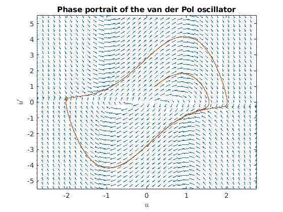
The first two lines define the van der Pol equation with μ = 2.3.
We call quiver with N as an argument, along with a vector argument that specifies the lower and upper limits on the x and y axes. Furthermore, we give further arguments for customizing the plot.
Once we have called quiver, we overlay the phase plane portraits of solutions obtained by specifying different initial conditions -- notice how the solutions follow the arrows of the quiver plot, then get attracted to the same limit cycle (regardless of whether we start inside or outside of the cycle).
 Phas portrait for the van der Pol equation with μ = 2,3, plotted with Chebfun.
N = chebop(0,20);
N.op = @(t,u) 0.05*diff(u,2) - (1-u^2)*diff(u) + u;
N.lbc = [3; 0];
u = N\0;
plot(u,'LineWidth', 3), ylim([-4 4]), grid on