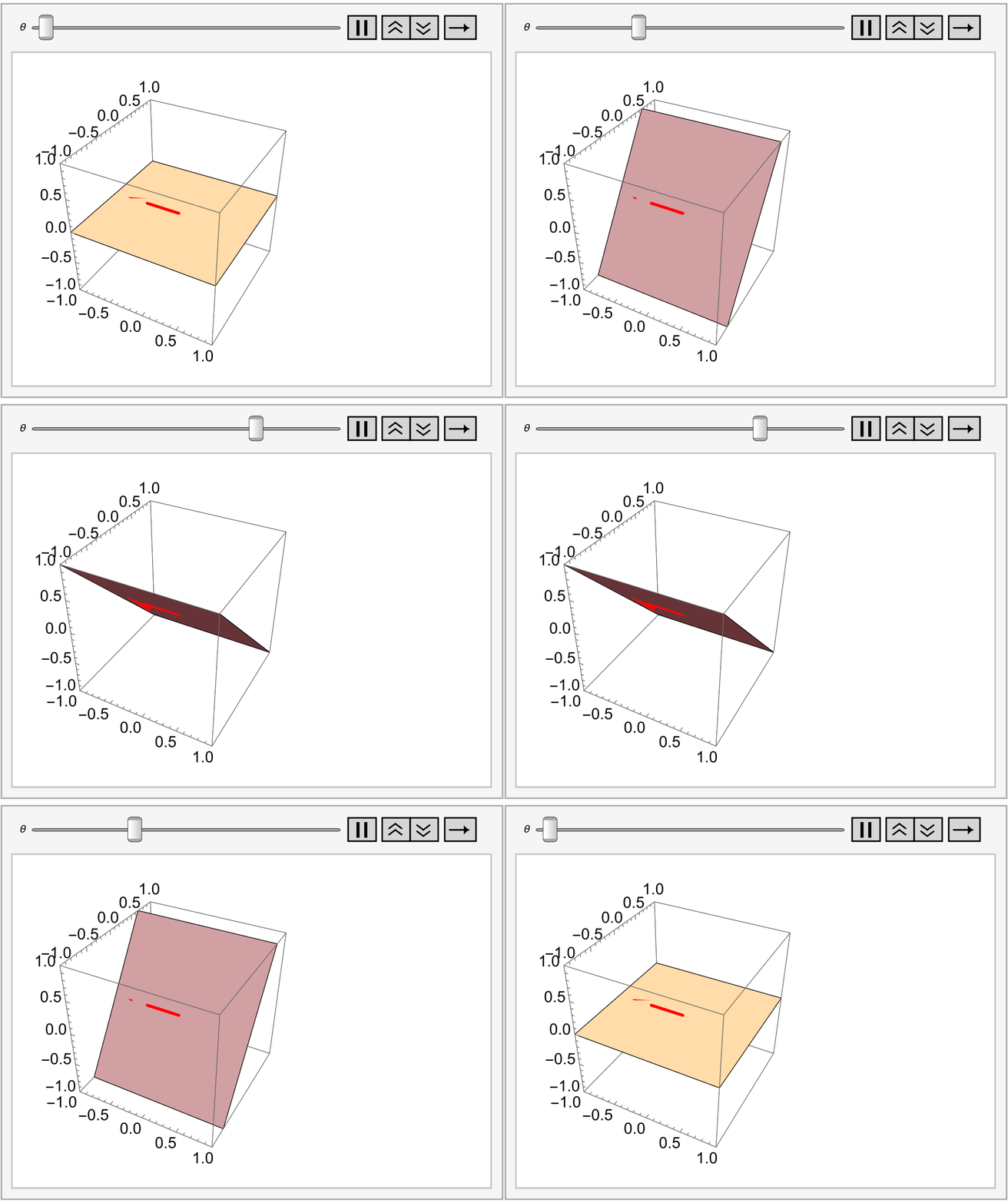
There are two kinds of matrix spaces: one is defined by a set of matrices of special type (considered in section), and another is associated with every matrix. This section is devoted to the latter case.
Matrix Spaces
We know from previous discussions that every real or complex n-dimensional vector space is isomorphic to ℝn or ℂn. This gives us the ground to consider linear transformations from one Euclidean Vector Space ℝn (or ℂn) into another one ℝm (or ℂm) instead of general finite dimensional vector spaces. Every linear transformation T: V ↦ W from one n-dimensional vectors space V into another m-dimensional vector space W is equivalent to a corresponding matrix transformation x ↦ Ax for some m×n matrix A for appropriate chosen bases. The inverse statement is obviously true because multiplication by a matrix defines a linear transformation.
Let A be an m-by-n matrix that maps \( \mathbb{R}^n \) into \( \mathbb{R}^m . \) So for every (colomn) vector \( {\bf x} = \left[ x_1 , x_2 , \ldots , x_n \right]^{\mathrm{T}} \) corresponds a vector \( {\bf A}\,{\bf x} \in \mathbb{R}^m . \)
Let V and U be vector spaces and \( T:\,U \to V \) be linear transformation. Then the set of all vectors of the form \( {\bf y} = {\bf A}\,{\bf x} \in V \) is called the range (or image) of T.
Theorem: Let V and U be vector spaces and \( T:\,U \to V \) be linear transformation. Then the range of T is a subspace of V.
Because \( T\left( 0U \right) = 0V, \) we have that \( 0V \in R(T) . \) Now let us choose two vectors \( {\bf x}, \, {\bf y} \in R(T) \) from the range and a scalar k. Then there exist two vectors u and v such that \( T({\bf u}) = {\bf x} \) and \( T({\bf v}) = {\bf y} . \) Hence, \( T({\bf u} + {\bf v}) = T({\bf u}) + T({\bf v}) = {\bf x} + {\bf y} \) and \( T(k{\bf u}) = k\, T({\bf u}) = k\, {\bf x} . \) Thus, \( T({\bf u} + {\bf v}) = T({\bf u}) + T({\bf v}) = {\bf x} + {\bf y} \in R(T) \) and \( T(k\,{\bf u}) = k \, T({\bf x}) = k\,{\bf x} \in R(T) , \) so R(T) is a subspace of V.
Recall that a set of vectors β is said to generate or span a vector space V if every element from V can be represented as a linear combination of vectors from β.
Theorem 2: A linear map T : 𝔽n ⇾ 𝔽m is onto if Im(T) = 𝔽m, so dim(Im(T)) = m. This means that the corresponding m×n matrix is of full row rank (= its rows are linearly independent).
Theorem 3: A linear map T : 𝔽n ⇾ 𝔽m is one-to-one if ker(T) = {0}, and it is onto if Range(T) = 𝔽m.
Theorem 4: A linear map T : 𝔽n ⇾ 𝔽m is bijection if and only if T sends a basis of the domain 𝔽n to a basis of the range 𝔽m.
Corollary 1: A linear map T : 𝔽n ⇾ 𝔽m is bijection if and only if dim(ker(T)) = 0 and dim(Im(T)) = m.
Corollary 2: A linear map T : 𝔽n ⇾ 𝔽m is bijection if and only if n = m and the matrix A representing T is invertible.
Corollary 3: A linear map T : 𝔽n ⇾ 𝔽n is onto if and only if for any spanning subset S of 𝔽n, we have that T(S) is a spanning subset of 𝔽n.
Theorem 5: A linear map T : 𝔽n ⇾ 𝔽m is onto if Im(T) = 𝔽m, so dim(Im(T)) = m. This means that the corresponding m×n matrix is of full row rank (= its rows are linearly independent).

