Introduction to Linear Algebra
Systems of Linear Equations
- Introduction
- Linear systems
- Vectors
- Linear combinations
- Matrices
- Planes in ℝ³
- Reduced Row-Echelon Form
- Equation A x = b
- Sensitivity of solutions
- Linear independence
- Plane transformations
- Space transformations
- Linear transformations
- Affine maps
- Exercises
- Answers
Matrix Algebra
- Introduction
- Manipulation of matrices
- Partitioned matrices
- Block matrices
- Matrix operators
- Determinants
- Cofactors
- Cramer's rule
- Equivalent matrices
- Elimination: A = L U
- PLU factorization
- Reflection
- Givens rotation
- Special matrices
- Exercises
- Answers
Vector Spaces
- Introduction
- Motivation
- Vector spaces
- Bases
- Dimension
- Coordinate systems
- Linear transformations
- Change of basis
- Matrix transformations
- Compositions
- Isomorphisms
- Dual transformations
- Quotient spaces
- Wedge products
- Rotors
Eigenvalues, Eigenvectors
- Introduction
- Characteristic polynomials
- Companion matrix
- Algebraic and geometric multiplicities
- Minimal polynomials
- Eigenspaces
- Where are eigenvalues?
- Eigenvalues of A B and B A
- Generalized eigenvectors
- Similarity
- Diagonalizability
- Self-adjoint operators
- Exercises
- Answers
Euclidean Spaces
- Introduction
- Dot product
- Euclidean space
- Bilinear transformations
- Norm and distance
- Matrix norms
- Dual norms
- Dual transformations
- Examples of transformations
- Orthogonality
- Gram--Schmidt Process
- Orthogonal matrices
- Self-adjoint matrices
- Unitary matrices
- Projection operators
- QR-decomposition
- Least Square Approximation
- Quadratic forms
- Exercises
- Answers
Matrix Decompositions
- Introduction
- 2D decomposition
- Projectors
- Direct-sum decompositions
- Cyclic decompositions
- Symmetric matrices
- Pseudoinverse
- URV-decomposition
- LU-decomposition
- QR-decomposition
- Cholesky decomposition
- Schur decomposition
- Positive matrices
- Roots
- Polar factorization
- Spectral decomposition
- CUR decomposition
- Exercises
- Answers
Tensors
- Introduction
- Circles along curves
- TNB frames
- Tensors
- Tensors in ℝ³
- Tensors & Mechanics
- Differential forms
- Calculus
- Answers
Applications
- Introduction
- GPS problem
- Poisson equation
- Graph theory
- Error correcting codes
- Electric circuits
- FSA
- Markov chains
- Cryptography
- Wave-length transfer matrix
- Computer graphics
- Linear Programming
- Hill's determinant
- Fibonacci matrices
- Discrete dynamic systems
- Discrete Fourier transform
- Fast Fourier transform
- Curve fitting
- Answers
Functions of Matrices
- Introduction
- Diagonalization
- Sylvester formula
- The Resolvent method
- Polynomial interpolation
- Positive matrices
- Roots <
- Pseudoinverse
- Exercises
- Answers
Miscellany
- Introduction
- Circles along curves
- TNB frames
- Differential forms
- Calculus
- Vector representations
- Matrix representations
- Change of basis
- Orthonormal Diagonalization
- Generalized inverse
- Differential forms
Preliminaries
- Complex Number Operations
- Sets
- Polynomials
- Polynomials and Matrices
- Computer solves Systems of Linear Equations
- Location of Eigenvalues
- Power Method
- Iterative Method
- Similarity and Diagonalization
Glossary
Reference

This Book is licensed under Creative Commons Attribution-NonCommercial-NoDerivs 3.0 Unported License
Electric Circuits
Introduction
Today more than ever, electronics are an integral part of our everyday lives. They contribute to every aspect of our way of life from lighting the space around our work environments, to exploring uncharted territories. But behind each and every electrical appliance or device, no matter what task it was designed for, lies a vast system of electrical components that must function as a whole. Each component (resistors, capacitors, inductors, etc.) has specifications of their own, as does the final product that they are a part of, so engineers must design their devices to meet not only their intended purpose, but so that the individual components are within their tolerances. Vital to this is the analysis of currents and voltages throughout the electrical circuit. (Tiang, 2001)
Linear algebra is an essential tool when working with electric circuits. The use of matrices is considered to be an integral concept utilized by electrical engineers. Most of computer applications are based on linear algebra including solutions of systems of linear equations. Aside from the traditional approach of evaluating circuits by looking at the left most and right most elements, there are many other choices when it comes to solving electric circuit problems. Initially, an individual can begin solving the circuit problem by looking at the output portion of the matter and work back towards the input portion of the circuit. In other words, there are multiple approaches to circuity problems, aside from a traditional approach of evaluating the circuit from looking at the leftmost elements to the rightmost elements.
Electrical elements are conceptual abstractions representing idealized electrical components, such as resistors, capacitors, and inductors, used in the analysis of electrical networks. All electrical networks can be analyzed as multiple electrical elements interconnected by wires.
A resistor is a passive two-terminal electrical component that implements electrical resistance as a circuit element. In electronic circuits, resistors are used to reduce current flow, adjust signal levels, to divide voltages, bias active elements, and terminate transmission lines, among other uses. The behavior of an ideal resistor is dictated by the relationship specified by Ohm's law:
The typical schematic diagram symbol for resistor is
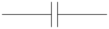
A capacitor is a passive two-terminal electrical component that stores potential energy in an electric field. The effect of a capacitor is known as capacitance. While some capacitance exists between any two electrical conductors in proximity in a circuit, a capacitor is a component designed to add capacitance to a circuit. The typical schematic diagram symbol for capacitor is
l2 = Graphics[{Thick, Line[{{1.5, -1}, {1.5, 1}}]}];
l3 = Graphics[{Thick, Line[{{-3, 0}, {1, 0}}]}];
l4 = Graphics[{Thick, Line[{{5.5, 0}, {1.5, 0}}]}];
Show[l1, l2, l3, l4]
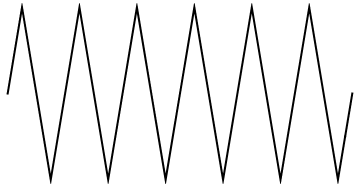
An inductor, also called a coil, choke or reactor, is a passive two-terminal electrical component that stores energy in a magnetic field when electric current flows through it. When the current flowing through an inductor changes, the time-varying magnetic field induces an electromotive force (e.m.f.) (voltage) in the conductor, described by Faraday's law of induction. An inductor is characterized by its inductance, which is the ratio of the voltage to the rate of change of current. In the International System of Units (SI), the unit of inductance is the henry (H) named for 19th century American scientist Joseph Henry (1797--1878).

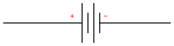
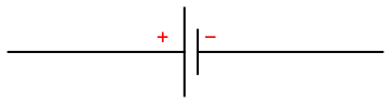
An electric battery is a device consisting of one or more electrochemical cells with external connections provided to power electrical devices such as flashlights, smartphones, and electric cars. When a battery is supplying electric power, its positive terminal is the cathode and its negative terminal is the anode. The terminal marked negative is the source of electrons that when connected to an external circuit will flow and deliver energy to an external device. The following symbol for a battery is used in a circuit diagram.
l2 = Graphics[{Thick, Line[{{1.6, -1}, {1.6, 1}}]}];
l3 = Graphics[{Thick, Line[{{-3, 0}, {1, 0}}]}];
l4 = Graphics[{Thick, Line[{{5.5, 0}, {1.9, 0}}]}];
l5 = Graphics[{Thick, Line[{{1.3, -0.5}, {1.3, 0.5}}]}];
l6 = Graphics[{Thick, Line[{{1.9, -0.5}, {1.9, 0.5}}]}];
txt1 = Graphics[Text[Style["+", FontSize -> 14, Red], {0.5, 0.4}]];
txt2 = Graphics[Text[Style["-", FontSize -> 14, Red], {2.2, 0.4}]];
Show[l1, l2, l3, l4, l5, l6, txt1, txt2]
l3 = Graphics[{Thick, Line[{{-3, 0}, {1, 0}}]}];
l4 = Graphics[{Thick, Line[{{5.5, 0}, {1.3, 0}}]}];
l5 = Graphics[{Thick, Line[{{1.3, -0.5}, {1.3, 0.5}}]}]; txt1 = Graphics[Text[Style["+", FontSize -> 18, Red], {0.5, 0.4}]];
txt2 = Graphics[Text[Style["-", FontSize -> 18, Red], {1.6, 0.4}]];
Show[l1, l3, l4, l5, txt1, txt2]
graph = Plot[-0.7*Sin[2*x], {x, -1.3, 1.3}, PlotStyle -> {Black, Thick}]
Show[circle, graph]
gap[l_: 1] := Line[l {{{0, 0}, {1/3, 0}}, {{2/3, 0}, {1, 0}}}];
battery[l_: 1] := {gap[ l], {Rectangle[l {1/3, -(2/3)}, l {1/3 + 1/9, 2/3}], Line[l {{2/3, -1}, {2/3, 1}}]}};
resistor[l_: 1, n_: 3] := Line[Table[{i l/(4 n), 1/3 Sin[i Pi/2]}, {i, 0, 4 n}]];
contact[l_: 1] := {gap[l], Map[{EdgeForm[Directive[Thick, Black]], FaceForm[White], Disk[#, l/30]} &, l {{1/3, 0}, {2/3, 0}}]} Options[display] = {Frame -> True, FrameTicks -> None, PlotRange -> All, GridLines -> Automatic, GridLinesStyle -> Directive[Orange, Dashed], AspectRatio -> Automatic};
display[d_, opts : OptionsPattern[]] := Graphics[Style[d, Thick], Join[FilterRules[{opts}, Options[Graphics]], Options[display]]]; at[position_, angle_: 0][obj_] := GeometricTransformation[obj, Composition[TranslationTransform[position], RotationTransform[angle]]]; label[s_String, color_: RGBColor[.3, .5, .8]] := Text@Style[s, FontColor -> color, FontFamily -> "Geneva", FontSize -> Large]; display[{connect[{{0, -2}, {0, -3}}], resistor[] // at[{0, -1}, 3 Pi/2], connect[{{0, -1}, {0, 0}}], connect[{{0, 0}, {3, 0}}], resistor[] // at[{3, 0}], connect[{{4, 0}, {7, 0}}], connect[{{0, 0}, {0, 3}}], connect[{{0, 3}, {1, 3}}], resistor[] // at[{1, 3}], connect[{{2, 3}, {5, 3}}], resistor[] // at[{5, 3}], connect[{{6, 3}, {7, 3}, {7, -1}}], resistor[] // at[{7, -1}, 3 Pi/2], connect[{{7, -2}, {7, -3}, {4, -3}}], battery[] // at[{4, -3}, Pi], connect[{{0, -3}, {3, -3}}], Text[Style["1300-W", FontSize -> 15], {1.5, 4}], Text[Style["Vacuum", FontSize -> 15], {1.5, 2}], Text[Style["80-W", FontSize -> 15], {5.5, 4}], Text[Style["Television", FontSize -> 15], {5.5, 2}], Text[Style["1500-W", FontSize -> 15], {8.5, -1.5}], Text[Style["Refrigerator", FontSize -> 15], {8.5, -2}], Text[Style["120-V", FontSize -> 15], {3.5, -4.5}], Text[Style["1250-W", FontSize -> 15], {-2, -1.5}], Text[Style["Dish Washer", FontSize -> 15], {-2, -2}], Text[Style["1400-W", FontSize -> 15], {3.5, 1}], Text[Style["Fan", FontSize -> 15], {3.5, -1}]}]
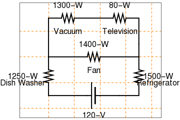
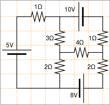
In order to find the current passing through the outlet, we need to find the current running through each appliance and the voltage at various places in the circuit.
The first step in analyzing this circuit is to find the resistance of each appliance. Using the information supplied by the manufacturer, the resistance for each appliance can be determined. Figure 2 shows the resistance of each appliance, and also the remaining unknown currents and voltages.
Here is another circuit:
Here is another circuit:
- Kirchhoff's current law (KCL): at any node (junction) in an electrical circuit, the sum of currents flowing into that node is equal to the sum of currents flowing out of that node
- Kirchhoff's voltage law (KVL): the sum of the emfs in any closed loop is equal to the sum of the potential drops in that loop.
- when we travel around a loop of the circuit, the algebraic sum of the volts has to be equal to zero;
- always start at the battery.
resistor[l_: 1, n_: 3] := Line[Table[{i l/(4 n), 1/3 Sin[i Pi/2]}, {i, 0, 4 n}]];
contact[l_: 1] := {gap[l], Map[{EdgeForm[Directive[Thick, Black]], FaceForm[White], Disk[#, l/30]} &, l {{1/3, 0}, {2/3, 0}}]};
Options[display] = {Frame -> True, FrameTicks -> None, PlotRange -> All, AspectRatio -> Automatic};
display[d_, opts : OptionsPattern[]] := Graphics[Style[d, Thick], Join[FilterRules[{opts}, Options[Graphics]], Options[display]]];
at[position_, angle_: 0][obj_] := GeometricTransformation[obj, Composition[TranslationTransform[position], RotationTransform[angle]]];
label[s_String, color_: RGBColor[.3, .5, .8]] := Text@Style[s, FontColor -> color, FontFamily -> "Times", FontSize -> Large];
display[{connect[{{0, -2}, {0, 1}, {1, 1}}], battery[] // at[{1, 1}], connect[{{2, 1}, {3, 1}, {3, 0}}], resistor[] // at[{3, 0}, 3 Pi/2], connect[{{3, -1}, {3, -2}, {2, -2}}], resistor[] // at[{1, -2}], connect[{{1, -2}, {0, -2}}], Text[Style["2\[CapitalOmega]", FontSize -> 30], {2.4, -0.5}], Text[Style["10 V", FontSize -> 30], {1.5, 0.3}], Text[Style["8\[CapitalOmega]", FontSize -> 30], {1.5, -1.3}]}]
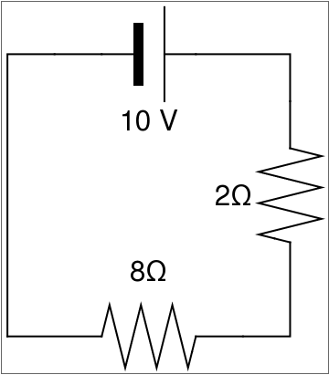
- Start from the battery.
- The current flow from the battery is clockwise. Therefore, we start on the + side: 10 v.
- Traveling clockwise to the 2 Ω: 10 v + 2 i.
- Traveling clockwise once again to the 8 Ω:10 v + 2 i + 8 i = 0.
- We have completed our equation because we have only one loop, so there is a single equation for voltage v and current i.
display[{connect[{{1, -2}, {0, -2}, {0, 1}, {1, 1}}], battery[] // at[{2, 1}, Pi], connect[{{2, 1}, {3, 1}, {3, 0}}], resistor[] // at[{3, 0}, 3 Pi/2], connect[{{3, -1}, {3, -2}, {2, -2}}], resistor[] // at[{1, -2}], connect[{{3, 1}, {4, 1}}], resistor[] // at[{4, 1}], connect[{{5, 1}, {6, 1}, {6, 0}}], resistor[] // at[{6, 0}, 3 Pi/2], connect[{{6, -1}, {6, -2}, {5, -2}}], battery[] // at[{4, -2}], connect[{{3, -2}, {4, -2}}], Text[Style["2\[CapitalOmega]", FontSize -> 20], {2.4, -0.5}], Text[Style["7\[CapitalOmega]", FontSize -> 20], {5.4, -0.5}], Text[Style["3\[CapitalOmega]", FontSize -> 20], {4.5, 0.3}], Text[Style["10 V", FontSize -> 20], {1.5, 0.3}], Text[Style["8\[CapitalOmega]", FontSize -> 20], {1.5, -1.3}], Text[Style["12 V", FontSize -> 20], {4.5, -1.3}]}]
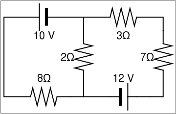
- Starting from the battery our direction is going from the - to the + position, counter clockwise. Therefore, we have a positive volt number: 12 v.
-
Traveling to the 2 Ω, we notice that the 2 Ω is being shared by
both circuits. Once again, we calculate by using the circuit that we are in
subtracted by the other circuit:
\[ _ 12\,v + 2 \left( i_1 - i_2 \right) , \]where i1 and i2 are currents in every loop, respectively.
-
Continuing on to 3 Ω:
\[ 12\,v + 2 \left( i_2 - i_1 \right) + 3\, i_2 . \]
-
Finally we approach 7 Ω, completing our i2 equation:
\[ \begin{split} 12\,v + 2 \left( i_2 - i_1 \right) + 3\,i_2 + 7\,i_2 &= 0, \\ -2\,i_1 + 12\,i_2 &= -12\,v . \end{split} \]
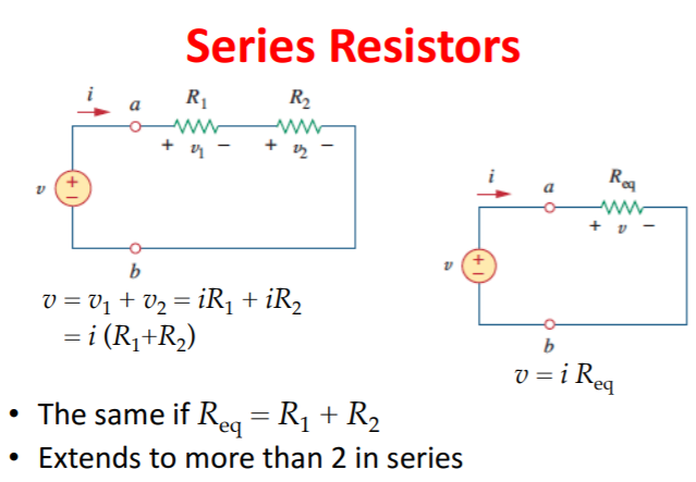
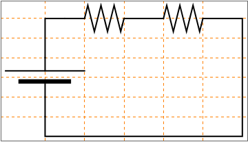
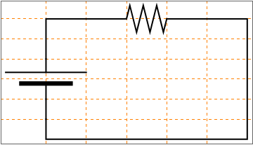
One of the basic fundamentals to simplifying and solving a circuit is to focus on multiple resistors that have connections with one another. Depending upon the configuration of the ladder network, the resistors in series can be added up to simplify the resistance in that certain region of the circuit.
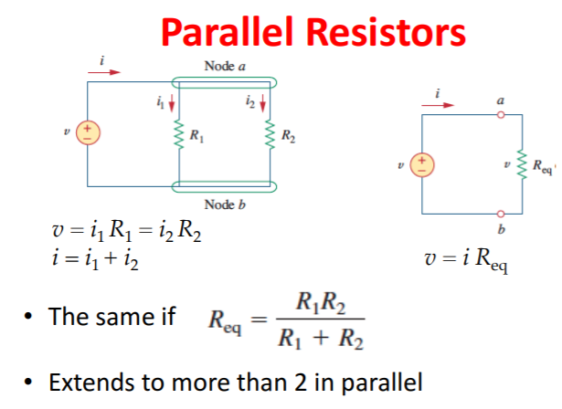
In addition, resistors in parallel can be combined by adding the inverse of all of the parallel resistances.
gap[l_: 1] := Line[l {{{0, 0}, {1/3, 0}}, {{2/3, 0}, {1, 0}}}]
battery[l_: 1] := {gap[ l], {Rectangle[l {1/3, -(2/3)}, l {1/3 + 1/9, 2/3}], Line[l {{2/3, -1}, {2/3, 1}}]}}
resistor[l_: 1, n_: 3] := Line[Table[{i l/(4 n), 1/3 Sin[i Pi/2]}, {i, 0, 4 n}]]
contact[l_: 1] := {gap[l], Map[{EdgeForm[Directive[Thick, Black]], FaceForm[White], Disk[#, l/30]} &, l {{1/3, 0}, {2/3, 0}}]}
Options[display] = {Frame -> True, FrameTicks -> None, PlotRange -> All, GridLines -> Automatic, GridLinesStyle -> Directive[Orange, Dashed], AspectRatio -> Automatic};
display[d_, opts : OptionsPattern[]] := Graphics[Style[d, Thick], Join[FilterRules[{opts}, Options[Graphics]], Options[display]]]
at[position_, angle_: 0][obj_] := GeometricTransformation[obj, Composition[TranslationTransform[position], RotationTransform[angle]]]
label[s_String, color_: RGBColor[.3, .5, .8]] := Text@Style[s, FontColor -> color, FontFamily -> "Geneva", FontSize -> Large];
display[{battery[] // at[{0, 0}, Pi/2], connect[{{0, 1}, {0, 2}, {3, 2}, {3, 1}}], resistor[] // at[{3, 0}, Pi/2], connect[{{3, 2}, {6, 2}, {6, 1}}], resistor[] // at[{6, 0}, Pi/2], connect[{{6, 0}, {6, -1}, {0, -1}, {0, 0}}], connect[{{3, 0}, {3, -1}}]}]
label[s_String, color_: RGBColor[.3, .5, .8]] := Text@Style[s, FontColor -> color, FontFamily -> "Geneva", FontSize -> Large];
display[{battery[] // at[{0, 0}, Pi/2], connect[{{0, 1}, {0, 2}, {3, 2}, {3, 1}}], resistor[] // at[{3, 0}, Pi/2], connect[{{3, 0}, {3, -1}, {0, -1}, {0, 0}}]}]
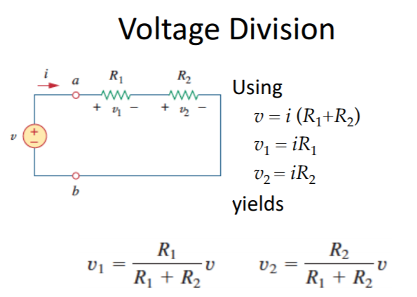
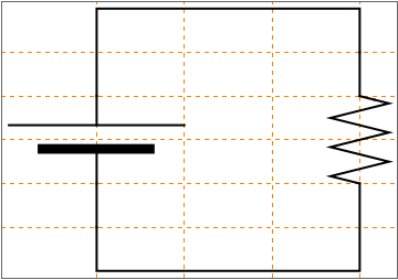
After the simplification of combining series and parallel resistors, there are operations in electrical engineering that can be used to solve for other elements in the circuit. For instance, having resistors in series enables the use of voltage division. Voltage division is a procedure that is used to solve for the voltage of a resistor (when that particular resistor is in series with another resistor in the circuit).
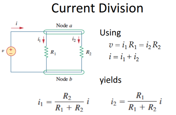
Moreover, resistors in parallel allows the use of an operation known as current division. Current division is a function that is used to solve for the current that passes through a resistor (when that particular resistor is connected in parallel with another resistor in the circuit).
The input voltage (v1) and the input current (i1) in an electrical circuit is set up in a matrix form that looks like \( \begin{bmatrix} v_1 \\ i_1 \end{bmatrix} . \) Meanwhile, the output voltage (v2) and the output current (i2) is set up in a column vector form that equates to \( \begin{bmatrix} v_2 \\ i_2 \end{bmatrix} . \) Taking a standard electrical circuit with a linear transformation is known as a transfer matrix, which is written as \( \begin{bmatrix} v_2 \\ i_2 \end{bmatrix} = {\bf A}\, \begin{bmatrix} v_1 \\ i_1 \end{bmatrix} . \)
It is entirely possible that an electrical engineer could find themselves faced with solving a ladder network, which links two circuits together that are connected in series with one another. The output of the first circuit in the network is subsequently used as the input to the next circuit that is in the network. In the figure pictured below, the circuit with resistor R1 is recognized as a series circuit and the circuit with resistor R2 is recognized as a shunt circuit.
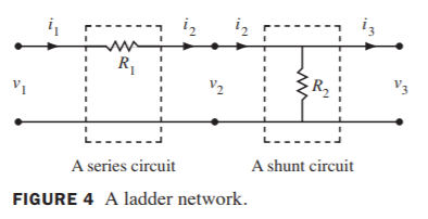
Given both of these circuits, the transfer matrices for each of the respective circuits are written as \( {\bf A}_1 = \begin{bmatrix} 1& -R_1 \\ 0&1 \end{bmatrix} \) (transfer matrix of series circuit) and \( {\bf A}_2 = \begin{bmatrix} 1& 0 \\ -1/R_2&1 \end{bmatrix} \) (transfer matrix of shunt circuit). Evidently, it is possible to solve through the transfer matrix (A1 for the series circuit and A2 for the shunt circuit) that epitomizes the figure of the ladder network that was just shown. After using an input vector x, the transfer matrix is illustrated as
Just like in this scenario, an electrical engineer must first find out if a network like the ladder network in figure four can be built. Assuming that the network can be created, the next step is to use matrix factorization on the transfer matrix in order to find the matrices that are connected to smaller circuits. The smaller circuits can then be used to compose the network or the smaller circuits may already be a part of a configuration such as a ladder network. In some cases, the transfer matrix can contain values that contain complex numbers. Ultimately, the goal is to try to build the network that the electrical engineer needs while expending the least number of electrical elements.
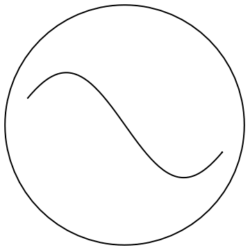
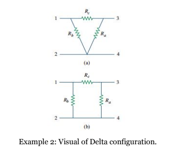
For the more daring electrical engineer, matrices can help simplify the most complex circuits that are non-linear, like a delta-delta transformer. A transformer is an electrical device that is designed on the basis of the concept of magnetic coupling. It uses magnetically coupled coils to transfer energy from one circuit to another. The transformer can be used for “stepping up” or “stepping down” AC voltages or currents. AC stands for alternating current and the voltage that was dealt with before is DC (directed current). Delta configuration represents the order of components, usually two grounded components, and one connection between them. Stating a delta-delta transformation essentially states that they are connected together.
gap[l_: 1] := Line[l {{{0, 0}, {1/3, 0}}, {{2/3, 0}, {1, 0}}}]
battery[l_: 1] := {gap[ l], {Rectangle[l {1/3, -(2/3)}, l {1/3 + 1/9, 2/3}], Line[l {{2/3, -1}, {2/3, 1}}]}}
resistor[l_: 1, n_: 3] := Line[Table[{i l/(4 n), 1/3 Sin[i Pi/2]}, {i, 0, 4 n}]]
contact[l_: 1] := {gap[l], Map[{EdgeForm[Directive[Thick, Black]], FaceForm[White], Disk[#, l/30]} &, l {{1/3, 0}, {2/3, 0}}]} Options[display] = {Frame -> True, FrameTicks -> None, PlotRange -> All, GridLines -> Automatic, GridLinesStyle -> Directive[Orange, Dashed], AspectRatio -> Automatic};
display[d_, opts : OptionsPattern[]] := Graphics[Style[d, Thick], Join[FilterRules[{opts}, Options[Graphics]], Options[display]]];
at[position_, angle_: 0][obj_] := GeometricTransformation[obj, Composition[TranslationTransform[position], RotationTransform[angle]]];
label[s_String, color_: RGBColor[.3, .5, .8]] := Text@Style[s, FontColor -> color, FontFamily -> "Geneva", FontSize -> Large];
display[{connect[{{0, 1}, {3.5, 1}}], resistor[] // at[{3.5, 1}], connect[{{4.5, 1}, {8, 1}}], connect[{{2.75, -0.75}, {4, -2}}], resistor[] // at[{2, 0}, 7 Pi/4], connect[{{1, 1}, {2, 0}}], connect[{{4, -2}, {5.25, -0.75}}], resistor[] // at[{5.25, -0.75}, Pi/4], connect[{{6, 0}, {7, 1}}], connect[{{0, -2}, {8, -2}}]}]
label[s_String, color_: RGBColor[.3, .5, .8]] := Text@Style[s, FontColor -> color, FontFamily -> "Geneva", FontSize -> Large];
display[{connect[{{0, 1}, {3.5, 1}}], resistor[] // at[{3.5, 1}], connect[{{4.5, 1}, {8, 1}}], connect[{{1, -1}, {1, -2}}], connect[{{1, 1}, {1, 0}}], connect[{{0, -2}, {8, -2}}], resistor[] // at[{1, 0}, 3 Pi/2], connect[{{7, 1}, {7, 0}}], connect[{{7, -1}, {7, -2}}], resistor[] // at[{7, 0}, 3 Pi/2]}]
Not all electrical engineering problems have numbers that can be solved, however that does not stop someone from making an equation for future use, once other values are known. In reality, this is actually a common practice for electrical engineers when the desired input and output is unknown.
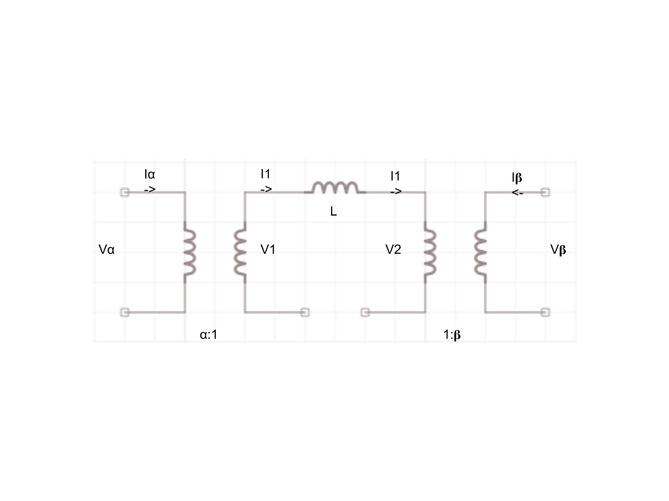
As stated before, a transformer's transfer energy comes from one circuit. Due to power conservation, the energy that may be lost or gain is still maintained within a ratio before the circuits, as shown below
The following formula was derived from the voltages on the two inductors multiple by the top inductor’s reactance
Now merge the above equations, and drive the V' and V'' from the circuit based on power conservation.
Plug and reduce, Therefore \( I_\alpha = \alpha^{-1} \left( \alpha^{-1} V_\alpha - \beta^{-1} V_\beta \right) = \alpha^{-2} V_\alpha L - (\alpha \beta )^{-1} V_\beta L . \)
Now from \( I_\beta \), it followsbecause
Therefore
div class = "math"> \[ -I_\beta = \beta^{-2} \left(V_\beta L \right) + \beta\alpha^{-1} \left(V_\alpha L\right) \]This can all be simply put into a matrix, for a quick solve once we have our values.
Now if even we needed to use a delta-delta transformer to step-up or step-down and voltage or current, we can just solve for this matrix with our arguments.
In conclusion, electrical engineers calculate current flow through electrical circuits. With the help of linear algebra, Kirchhoff's voltage law, and Ohm’s law, one can easily solve for the value our unknown variables within a circuit. As long as the basic assumption of network flow is true, linear algebra will help make the problem easier to solve.
▢ Syntax: connect[{{x1, y1}, {x2, y2}, ...{xn, yn}}]
▢ Syntax: resistor[]//at[{x, y}, Θ]
▢ Syntax: coil[]//at[{x, y}, Θ]
▢ Syntax: capacitor[]//at[{x, y}, Θ]
▢ Syntax: battery[]//at[{x, y}, \[CapitalTheta]]
Options[display] = {Frame -> True, FrameTicks -> None, PlotRange -> All, GridLines -> Automatic, GridLinesStyle -> Directive[Orange, Dashed], AspectRatio -> Automatic};
▢ Syntax: at[{x, y}, Θ]
gap[l_: 1] := Line[l {{{0, 0}, {1/3, 0}}, {{2/3, 0}, {1, 0}}}]
resistor[l_: 1, n_: 3] := Line[Table[{i l/(4 n), 1/3 Sin[i Pi/2]}, {i, 0, 4 n}]
battery[l_: 1] := {gap[ l], {Rectangle[l {1/3, -(2/3)}, l {1/3 + 1/9, 2/3}], Line[l {{2/3, -1}, {2/3, 1}}]}}
contact[l_: 1] := {gap[l], Map[{EdgeForm[Directive[Thick, Black]], FaceForm[White], Disk[#, l/30]} &, l {{1/3, 0}, {2/3, 0}}]}
Options[display] = {Frame -> True, FrameTicks -> None, PlotRange -> All, GridLines -> Automatic, GridLinesStyle -> Directive[Orange, Dashed], AspectRatio -> Automatic};
display[d_, opts : OptionsPattern[]] := Graphics[Style[d, Thick], Join[FilterRules[{opts}, Options[Graphics]], Options[display]]]
at[position_, angle_: 0][obj_] := GeometricTransformation[obj, Composition[TranslationTransform[position], RotationTransform[angle]]]
label[s_String, color_: RGBColor[.3, .5, .8]] := Text@Style[s, FontColor -> color, FontFamily -> "Geneva", FontSize -> Large];
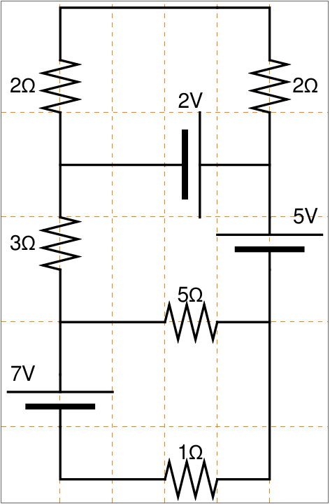
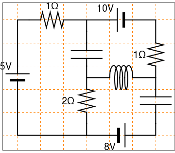
display[{battery[] // at[{0, -1}, Pi/2],
connect[{{0, 0}, {0, 2}, {1, 2}}], resistor[] // at[{1, 2}],
connect[{{2, 2}, {3, 2}, {3, 1}}], resistor[] // at[{3, 1}, 3 Pi/2],
connect[{{3, 0}, {3, -1}}], resistor[] // at[{3, -1}, 3 Pi/2], connect[{{2, -3}, {3, -3}, {3, -2}}],
connect[{{2, -3}, {0, -3}, {0, -1}}], connect[{{3, 2}, {4, 2}}],
battery[] // at[{5, 2}, Pi], connect[{{5, 2}, {6, 2}}],
battery[] // at[{4, -3}, 0], connect[{{3, -3}, {4, -3}}],
connect[{{5, -3}, {6, -3}, {6, -2}}],
resistor[] // at[{6, -1}, 3 Pi/2], connect[{{6, -1}, {6, 0}}],
resistor[] // at[{6, 1}, 3 Pi/2], connect[{{6, 2}, {6, 1}}],
connect[{{3, -0.5}, {4, -0.5}}], resistor[] // at[{4, -0.5}],
connect[{{5, -0.5}, {6, -0.5}}],
Text[Style["5V", FontSize -> 18], {-0.5, 0}],
Text[Style["10V", FontSize -> 18], {3.7, 2.5}],
Text[Style["8V", FontSize -> 18], {4, -3.5}],
Text[Style["1\[CapitalOmega]", FontSize -> 18], {1.5, 2.7}],
Text[Style["3\[CapitalOmega]", FontSize -> 18], {2.3, 0.5}],
Text[Style["1\[CapitalOmega]", FontSize -> 18], {5.3, 0.5}],
Text[Style["2\[CapitalOmega]", FontSize -> 18], {2.2, -1.5}],
Text[Style["4\[CapitalOmega]", FontSize -> 18], {4.4, 0.2}],
Text[Style["2\[CapitalOmega]", FontSize -> 18], {5.2, -1.5}]}]
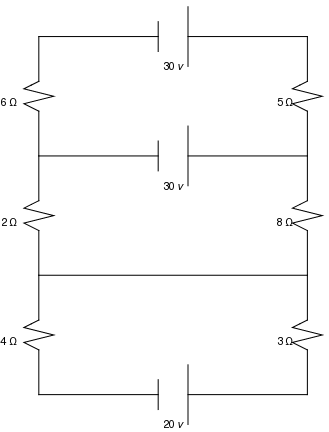
l2 = Line[{{2, 0.2}, {2.8, 0.2}}];
l3 = Line[{{1, 1}, {2.8, 1}}];
l4 = Line[{{1, 1.8}, {1.8, 1.8}}];
l5 = Line[{{2, 1.8}, {2.8, 1.8}}];
l6 = Line[{{1, 2.6}, {1.8, 2.6}}];
l7 = Line[{{2, 2.6}, {2.8, 2.6}}];
l8 = Line[{{1.8, 0.1}, {1.8, 0.3}}];
l9 = Line[{{2, 0}, {2, 0.4}}];
l10 = Line[{{1.8, 1.7}, {1.8, 1.9}}];
l11 = Line[{{2, 1.6}, {2, 2}}];
l12 = Line[{{1.8, 2.5}, {1.8, 2.7}}];
l13 = Line[{{2, 2.4}, {2, 2.8}}];
h = Line[{{1, 0.2}, {1, 0.5}}];
h2 = Line[{{1, 0.7}, {1, 1}}];
h3 = Line[{{2.8, 0.2}, {2.8, 0.5}}];
h4 = Line[{{2.8, 0.7}, {2.8, 1}}];
h5 = Line[{{1, 1}, {1, 1.3}}];
h6 = Line[{{1, 1.5}, {1, 1.8}}];
h7 = Line[{{2.8, 1}, {2.8, 1.3}}];
h8 = Line[{{2.8, 1.5}, {2.8, 1.8}}];
h9 = Line[{{1, 1.8}, {1, 2.1}}];
h10 = Line[{{1, 2.3}, {1, 2.6}}];
h11 = Line[{{2.8, 1.8}, {2.8, 2.1}}];
h12 = Line[{{2.8, 2.3}, {2.8, 2.6}}];
saw = Line[{{1, 0.5}, {0.9, 0.55}, {1.1, 0.6}, {0.9, 0.65}, {1, 0.7}}];
saw2 = Line[{{2.8, 0.5}, {2.7, 0.55}, {2.9, 0.6}, {2.7, 0.65}, {2.8, 0.7}}];
saw3 = Line[{{1, 1.3}, {0.9, 1.35}, {1.1, 1.4}, {0.9, 1.45}, {1, 1.5}}];
saw4 = Line[{{2.8, 1.3}, {2.7, 1.35}, {2.9, 1.4}, {2.7, 1.45}, {2.8, 1.5}}];
saw5 = Line[{{1, 2.1}, {0.9, 2.15}, {1.1, 2.2}, {0.9, 2.25}, {1, 2.3}}];
saw6 = Line[{{2.8, 2.1}, {2.7, 2.15}, {2.9, 2.2}, {2.7, 2.25}, {2.8, 2.3}}];
Graphics[{{l, Text[20 v, {1.9, 0}]}, {l2}, {l3}, {l4, Text[30 v, {1.9, 1.6}]}, {l5}, {l6}, {l7}, {l8, Text[30 v, {1.9, 2.4}]}, {l9}, {l10}, {l11}, {l12}, {l13}, {h}, {h2}, {h3}, {h4}, \ {h5}, {h6}, {h7}, {h8}, {h9}, {h10}, {h11}, {h12}, {saw, Text[4 \[CapitalOmega], {0.8, 0.56}]}, {saw2, Text[3 \[CapitalOmega], {2.65, 0.56}]}, {saw3, Text[2 \[CapitalOmega], {0.8, 1.36}]}, {saw4, Text[8 \[CapitalOmega], {2.65, 1.36}]}, {saw5, Text[6 \[CapitalOmega], {0.8, 2.16}]}, {saw6, Text[5 \[CapitalOmega], {2.65, 2.16}]}}]
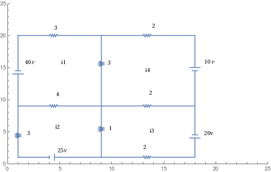
p2 = ListLinePlot[{{4, 0.75}, {4, 1.25}}, PlotRange -> {{0, 25}, {0, 25}}];
p3 = ListLinePlot[{{1, 1}, {1, 4}, \!\(\* TagBox[ FrameBox["\[Ellipsis]"], "Placeholder"]\)}, PlotRange -> {{0, 25}, {0, 25}}];
p4 = ListLinePlot[{{4.5, 0.5}, {4.5, 1.50}, \!\(\* TagBox[ FrameBox["\[Ellipsis]"], "Placeholder"]\)}, PlotRange -> {{0, 25}, {0, 25}}];
p5 = ListLinePlot[{{4.5, 1}, {13, 1}, \!\(\* TagBox[ FrameBox["\[Ellipsis]"], "Placeholder"]\)}, PlotRange -> {{0, 25}, {0, 25}}];
p6 = ListLinePlot[{{9, 1}, {9, 5}, \!\(\* TagBox[ FrameBox["\[Ellipsis]"], "Placeholder"]\)}, PlotRange -> {{0, 25}, {0, 25}}];
p7 = ListLinePlot[{{13.9, 1}, {18, 1}, {18, 1}, {18, 4}}, PlotRange -> {{0, 25}, {0, 25}}];
p8 = ListLinePlot[{{17.5, 4}, {18.5, 4}, \!\(\* TagBox[ FrameBox["\[Ellipsis]"], "Placeholder"]\)}, PlotRange -> {{0, 25}, {0, 25}}];
p9 = ListLinePlot[{{17.75, 4.5}, {18.25, 4.5}, \!\(\* TagBox[ FrameBox["\[Ellipsis]"], "Placeholder"]\)}, PlotRange -> {{0, 25}, {0, 25}}];
p10 = ListLinePlot[{{18, 4.5}, {18, 9}, \!\(\* TagBox[ FrameBox["\[Ellipsis]"], "Placeholder"]\)}, PlotRange -> {{0, 25}, {0, 25}}];
m1 = ListLinePlot[{{13, 1}, {13.1, 1.2}, {13.2, .8}, {13.3, 1.2}, {13.4, .8}, {13.5, 1.2}, {13.6, .8}, {13.7, 1.2}, {13.8, 1}}, PlotRange -> {{0, 25}, {0, 25}}];
m2 = ListLinePlot[{{9, 5}, {8.8, 5.1}, {9.2, 5.2}, {8.8, 5.3}, {9.2, 5.4}, {8.8, 5.5}, {9.2, 5.6}, {8.8, 5.7}, {9.0, 5.8}}, PlotRange -> {{0, 25}, {0, 25}}];
m3 = ListLinePlot[{{1, 4}, {.8, 4.1}, {1.2, 4.2}, {.8, 4.3}, {1.2, 4.4}, {.8, 4.5}, {1.2, 4.6}, {.8, 4.7}, {1.0, 4.8}}, PlotRange -> {{0, 25}, {0, 25}}];
p11 = ListLinePlot[{{1, 4.8}, {1, 9}}, PlotRange -> {{0, 25}, {0, 25}}];
p12 = ListLinePlot[{{1, 9}, {5, 9}, \!\(\* TagBox[ FrameBox["\[Ellipsis]"], "Placeholder"]\)}, PlotRange -> {{0, 25}, {0, 25}}];
m4 = ListLinePlot[{{4, 9}, {4.1, 9.2}, {4.2, 8.8}, {4.3, 9.2}, {4.4, 8.8}, {4.5, 9.2}, {4.6, 8.8}, {4.7, 9.2}, {4.8, 9}}, PlotRange -> {{0, 25}, {0, 25}}];
p12 = ListLinePlot[{{4.8, 9}, {9, 9}, \!\(\* TagBox[ FrameBox["\[Ellipsis]"], "Placeholder"]\)}, PlotRange -> {{0, 25}, {0, 25}}]; p13 = ListLinePlot[{{9, 9}, {9, 5.8}}, PlotRange -> {{0, 25}, {0, 25}}];
p14 = ListLinePlot[{{1, 9}, {4, 9}, \!\(\* TagBox[ FrameBox["\[Ellipsis]"], "Placeholder"]\)}, PlotRange -> {{0, 25}, {0, 25}}];
p15 = ListLinePlot[{{1, 9}, {1, 14}}, PlotRange -> {{0, 25}, {0, 25}}];
p16 = ListLinePlot[{{0.5, 14}, {1.5, 14}, \!\(\* TagBox[ FrameBox["\[Ellipsis]"], "Placeholder"]\)}, PlotRange -> {{0, 25}, {0, 25}}];
p17 = ListLinePlot[{{.75, 14.50}, {1.25, 14.50}, \!\(\* TagBox[ FrameBox["\[Ellipsis]"], "Placeholder"]\)}, PlotRange -> {{0, 25}, {0, 25}}];
p18 = ListLinePlot[{{1, 14.50}, {1, 20}, \!\(\* TagBox[ FrameBox["\[Ellipsis]"], "Placeholder"]\)}, PlotRange -> {{0, 25}, {0, 25}}];
p19 = ListLinePlot[{{1, 20}, {4, 20}, \!\(\* TagBox[ FrameBox["\[Ellipsis]"], "Placeholder"]\)}, PlotRange -> {{0, 25}, {0, 25}}];
m5 = ListLinePlot[{{4, 20}, {4.1, 20.2}, {4.2, 19.8}, {4.3, 20.2}, {4.4, 19.8}, {4.5, 20.2}, {4.6, 19.8}, {4.7, 20.2}, {4.8, 20}}, PlotRange -> {{0, 25}, {0, 25}}];
p20 = ListLinePlot[{{4.8, 20}, {9, 20}, \!\(\* TagBox[ FrameBox["\[Ellipsis]"], "Placeholder"]\)}, PlotRange -> {{0, 25}, {0, 25}}];
p21 = ListLinePlot[{{9, 20}, {9, 16}, \!\(\* TagBox[ FrameBox["\[Ellipsis]"], "Placeholder"]\)}, PlotRange -> {{0, 25}, {0, 25}}];
m6 = ListLinePlot[{{9, 16}, {8.8, 15.9}, {9.2, 15.8}, {8.8, 15.7}, {9.2, 15.6}, {8.8, 15.5}, {9.2, 15.4}, {8.8, 15.3}, {9.0, 15.2}}, PlotRange -> {{0, 25}, {0, 25}}];
p22 = ListLinePlot[{{9, 15.2}, {9, 9}, \!\(\* TagBox[ FrameBox["\[Ellipsis]"], "Placeholder"]\)}, PlotRange -> {{0, 25}, {0, 25}}];
p23 = ListLinePlot[{{9, 9}, {13, 9}, \!\(\* TagBox[ FrameBox["\[Ellipsis]"], "Placeholder"]\)}, PlotRange -> {{0, 25}, {0, 25}}];
m7 = ListLinePlot[{{13, 9}, {13.1, 9.2}, {13.2, 8.8}, {13.3, 9.2}, {13.4, 8.8}, {13.5, 9.2}, {13.6, 8.8}, {13.7, 9.2}, {13.8, 9}}, PlotRange -> {{0, 25}, {0, 25}}];
p24 = ListLinePlot[{{13.8, 9}, {18, 9}, \!\(\* TagBox[ FrameBox["\[Ellipsis]"], "Placeholder"]\)}, PlotRange -> {{0, 25}, {0, 25}}];
p25 = ListLinePlot[{{9, 20}, {13, 20}, \!\(\* TagBox[ FrameBox["\[Ellipsis]"], "Placeholder"]\)}, PlotRange -> {{0, 25}, {0, 25}}];
m8 = ListLinePlot[{{13, 20}, {13.1, 20.2}, {13.2, 19.8}, {13.3, 20.2}, {13.4, 19.8}, {13.5, 20.2}, {13.6, 19.8}, {13.7, 20.2}, {13.8, 20}}, PlotRange -> {{0, 25}, {0, 25}}];
p26 = ListLinePlot[{{13.8, 20}, {18, 20}, \!\(\* TagBox[ FrameBox["\[Ellipsis]"], "Placeholder"]\)}, PlotRange -> {{0, 25}, {0, 25}}];
p27 = ListLinePlot[{{18, 20}, {18, 15}, \!\(\* TagBox[ FrameBox["\[Ellipsis]"], "Placeholder"]\)}, PlotRange -> {{0, 25}, {0, 25}}];
p28 = ListLinePlot[{{17.5, 15}, {18.5, 15}, \!\(\* TagBox[ FrameBox["\[Ellipsis]"], "Placeholder"]\)}, PlotRange -> {{0, 25}, {0, 25}}];
p29 = ListLinePlot[{{17.75, 14.5}, {18.25, 14.5}, \!\(\* TagBox[ FrameBox["\[Ellipsis]"], "Placeholder"]\)}, PlotRange -> {{0, 25}, {0, 25}}];
p30 = ListLinePlot[{{18, 14.5}, {18, 9}, \!\(\* TagBox[ FrameBox["\[Ellipsis]"], "Placeholder"]\)}, PlotRange -> {{0, 25}, {0, 25}}];
Show[p1, p2, p3, p4, p5, p6, m1, p7, p8, p9, p10, m2, m3, p11, p12, \ m4, p13, p14, p15, p16, p17, p18, m5, p19, p20, p21, m6, p22, p23, \ m7, p24, m8, p25, p26, p27, p28, p29, p30]
gap[l_: 1] := Line[l {{{0, 0}, {1/3, 0}}, {{2/3, 0}, {1, 0}}}];
battery[l_: 1] := {gap[ l], {Rectangle[l {1/3, -(2/3)}, l {1/3 + 1/9, 2/3}], Line[l {{2/3, -1}, {2/3, 1}}]}};
resistor[l_: 1, n_: 3] := Line[Table[{i l/(4 n), 1/3 Sin[i Pi/2]}, {i, 0, 4 n}]];
contact[l_: 1] := {gap[l], Map[{EdgeForm[Directive[Thick, Black]], FaceForm[White], Disk[#, l/30]} &, l {{1/3, 0}, {2/3, 0}}]} Options[display] = {Frame -> True, FrameTicks -> None, PlotRange -> All, GridLines -> Automatic, GridLinesStyle -> Directive[Orange, Dashed], AspectRatio -> Automatic};
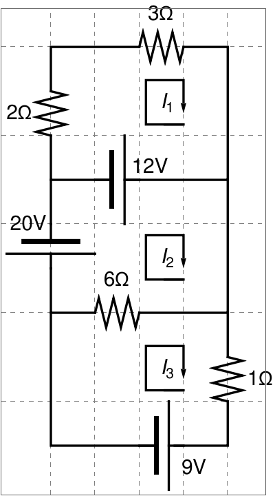
display[d_, opts : OptionsPattern[]] := Graphics[Style[d, Thick], Join[FilterRules[{opts}, Options[Graphics]], Options[display]]]; at[position_, angle_: 0][obj_] := GeometricTransformation[obj, Composition[TranslationTransform[position], RotationTransform[angle]]]; label[s_String, color_: RGBColor[.3, .5, .8]] := Text@Style[s, FontColor -> color, FontFamily -> "Times", FontSize -> Large]; display[{battery[] // at[{3, 4}, Pi], connect[{{0, 3}, {0, 4}, {2, 4}}], resistor[] // at[{0, 3}, 3 Pi/2], connect[{{0, 2}, {0, 0}}], resistor[] // at[{0, 0}, 3 Pi/2], connect[{{0, -1}, {0, -3}}], resistor[] // at[{0, -3}, 3 Pi/2], connect[{{0, -4}, {0, -5}, {2, -5}}], battery[] // at[{3, -5}, Pi], connect[{{3, -5}, {5, -5}, {5, -4}}], resistor[] // at[{5, -3}, 3 Pi/2], connect[{{5, -3}, {5, -1}}], resistor[] // at[{5, 0}, 3 Pi/2], connect[{{5, 0}, {5, 2}}], resistor[] // at[{5, 3}, 3 Pi/2], connect[{{5, 3}, {5, 4}, {3, 4}}], connect[{{0, 1}, {2, 1}}], resistor[] // at[{2, 1}], connect[{{3, 1}, {5, 1}}], connect[{{0, -2}, {1, -2}}], battery[] // at[{1, -2}], connect[{{2, -2}, {3, -2}}], resistor[] // at[{3, -2}], connect[{{4, -2}, {5, -2}}], Circle[{2.5, 2.5}, 0.5, {Pi/3, 7 Pi/4}], Arrow[{{2.87, 2.12}, {3.1, 2.5}}], Text[Style["I", FontSize -> 15, FontFamily -> "Times New Roman", FontSlant -> Italic], {2.5, 2.5}], Text[Style["1", FontSize -> 10, FontFamily -> "Times New Roman", FontSlant -> Italic], {2.65, 2.4}], Circle[{2.5, -0.5}, 0.5, {Pi/3, 7 Pi/4}], Arrow[{{2.87, -0.88}, {3.1, -0.5}}], Text[Style["I", FontSize -> 15, FontFamily -> "Times New Roman", FontSlant -> Italic], {2.5, -0.5}], Text[Style["2", FontSize -> 10, FontFamily -> "Times New Roman", FontSlant -> Italic], {2.65, -0.6}], Circle[{2.5, -3.5}, 0.5, {Pi/3, 7 Pi/4}], Arrow[{{2.87, -3.88}, {3.1, -3.5}}], Text[Style["I", FontSize -> 15, FontFamily -> "Times New Roman", FontSlant -> Italic], {2.5, -3.5}], Text[Style["3", FontSize -> 10, FontFamily -> "Times New Roman", FontSlant -> Italic], {2.65, -3.6}], Text[Style["30-V", FontSize -> 15], {3.2, 4.5}], Text[Style["4\[CapitalOmega]", FontSize -> 15], {4.3, 2.5}], Text[Style["1\[CapitalOmega]", FontSize -> 15], {4.3, -0.5}], Text[Style["1\[CapitalOmega]", FontSize -> 15], {4.3, -3.5}], Text[Style["4\[CapitalOmega]", FontSize -> 15], {0.7, 2.5}], Text[Style["1\[CapitalOmega]", FontSize -> 15], {0.7, -0.5}], Text[Style["1\[CapitalOmega]", FontSize -> 15], {0.7, -3.5}], Text[Style["5-V", FontSize -> 15], {1.5, -3.3}], Text[Style["1\[CapitalOmega]", FontSize -> 15], {3.5, -2.8}], Text[Style["3\[CapitalOmega]", FontSize -> 15], {2.5, 0.4}], Text[Style["20-V", FontSize -> 15], {1.8, -5.5}]}]


- Linear Algebra in Electrical Circuits
- Nodal Voltage Analysis of Electric Circuits
- Application of Linear Algebra in Electric CircuitsSeamleng Taing, 2001.
- James A. Svoboda, Richard C. Dorf, Introduction to Electric Circuits, 9th Edition, 2013, ISBN: 978-1-118-47750-2
- James A. Svoboda, Richard C. Dorf, Introduction to Electric Circuits, 8th Edition,