Preface

This section discusses differential equation used to model vibration of springs,

Pendulum Equation with Resistance

The pendulum equation can be also derived from the principle of angular momentum, which states that the time rate of change of angular momentum about any point is equal to the moment of the resultant force about that point. The position of the pendulum is described by the angle θ between the rod and the downward vertical direction, with the counterclockwise direction taken as positive. The gravitational force mg acts downward, while the damping force \( c \left\vert {\text d}\theta /{\text d}t \right\vert , \) where c is positive, is always oppose to the direction of motion. Here we take the damping force proportional to the velocity for simplicity; later we will discuss more realistic case.

Since the angular momentum about the origin is \( m\ell^2 \left( {\text d}\theta /{\text d}t \right) , \) the governing equation becomes

The resistance of the air acts on both the pendulum ball and the pendulum wire. It causes the amplitude to decrease with time and increases the period of oscillation slightly. The drag force is proportional to the velocity for values of the Reynolds number of the order 1 or less. For values of the Reynolds number of order \( 10^3 \) to \( 10^5 , \) the force is proportional to the square of the velocity. The maximum Reynolds number based on diameter for the ball is 1100, where the quadratic force law should apply, while the maximum value based on the diameter of a wire is about 6, where the linear force law should prevail.

Since the damping force is neither linear nor quadratic, but rather a combination of the two, it makes sense to establish a damping function which contains both effects simultaneously. Therefore, the pendulum equation becomes

where the linear damping coefficient \( \alpha = \kappa /m , \) describes air resistance due to the wire, the quadratic damping coefficient β is due to air drag on the pendulum bob, and the third damping term \( \quad \epsilon = c\ell /(2m) \) is necessary for taking into count the bearing, which is subject to dry friction (Coulomb damping). Here \( \quad \omega_0 = \left( g/\ell \right)^{1/2} ,\) and \( \mbox{sign}(x) = \begin{cases} 1, & \ x>0, \\ -1, & \ x<0. \end{cases} \)

Analysis of the experimental data gives the following values of the parameters (Robert A. Nelson and M.G. Olsson, "The pendulum---rich physics from a simple system," American Journal of Physics, Vol. 54, No 2, 112--121, 1986):

In order to find out the relationship between the angle of the pendulum and time t, a good way is to plot θ against t. In order to make the plot, first solve the differential equation with the command NDSolve.

This can be done by assigning constant values to α, ε and ω when using the NDSolve command, getting three different functions in respect to three different α values, and using the Plot command to plot the three functions in one graph

numsol1 =
  NDSolve[{y''[x] == -10*2*y'[x] - Sin[y[x]], y[0] == 0.7, y'[0] == 0}, y[x], {x, 0, 1000}]
numsol2 =
  NDSolve[{y''[x] == -1*2*y'[x] - Sin[y[x]], y[0] == 0.7, y'[0] == 0}, y[x], {x, 0, 1000}]
numsol3 =
  NDSolve[{y''[x] == -0.1*2*y'[x] - Sin[y[x]], y[0] == 0.7, y'[0] == 0}, y[x], {x, 0, 1000}]
Plot[Evaluate[y[x] /. {numsol1, numsol2, numsol3}], {x, 0, 100}, PlotRange -> All, PlotStyle -> {GrayLevel[0.1], Dashed, Thick}, AxesLabel -> {"t", "\[Theta]"}, PlotLegends -> {"\[Alpha]=10", "\[Alpha]=1", "\[Alpha]=0.1"}]

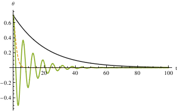
Another method is to set up a function that takes θ₀, ω₀, α, ε and tmax as inputs and outputs for a function of θ

DampedDrivenPendulumFunction2[{\[Theta]0_, \[Omega]0_}, \[Alpha]_, \ \[Epsilon]_, tmax_] :=
Module[{\[Theta]}, \[Theta] /. First[ NDSolve[{ \[Theta]''[t] == -Sin[\[Theta][t]] - 2 \[Alpha] \[Theta]'[ t] - \[Epsilon] Sign[\[Theta]'[t]] (\[Theta]'[t])^2, \[Theta][0] == \[Theta]0, \[Theta]'[0] == \[Omega]0}, \[Theta], {t, 0, tmax}

Plot[{DampedDrivenPendulumFunction2[{0.7, 0}, 0.1, 0, 100][x], DampedDrivenPendulumFunction2[{0.7, 0}, 1, 0, 100][x], DampedDrivenPendulumFunction2[{0.7, 0}, 10, 0, 100][x]}, {x, 0, 100}, PlotLegends -> "Expressions", PlotRange -> Full, PlotStyle -> {Thick, Automatic, Dashed}, AspectRatio -> 1.0]

The third method presented here is very different from the first and the second: we create a loop to add solutions into a list.

\[Epsilon] = 0; g = 9.8; \[Omega]0 = 1;

listofsolutions = {};

listofvaluesforalpha = {.1, 1, 10};

Numerically solve the corresponding second order differential equation, leaving alpha as a variable:

pendulumeq = \[Theta]''[t] + 2*\[Alpha] \[Theta]'[ t] + \[Epsilon] Sign[\[Theta]'[ t]]*((\[Theta]'[t])^2) + (\[Omega]0^2)*Sin[\[Theta][t]] == 0;

Get distinct equations for the different values of \[Alpha] and add them to the listofsolutions:

counter = 1;

While[counter <= Length[listofvaluesforalpha], AppendTo[listofsolutions, NDSolve[{Evaluate[ pendulumeq /. {\[Alpha] -> listofvaluesforalpha[[counter]]}], \[Theta][ 0] == .7, \[Theta]'[0] == 0}, \[Theta][t], {t, 0, 100}]]; counter++]

Plot[Evaluate[theta[t] /. listofsolutions], {t, 0, 50}, PlotRange -> All]

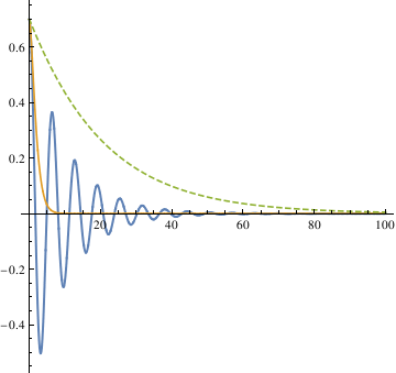
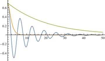
The three different methods all get the same result, from which we can see that the largest damping coefficient does not stop the pendulum the fastest. So the qualitative difference among the three different coefficients is that when α is 0.1, the pendulum oscillates (crosses 0). In other cases, the pendulum does not oscillate (does not cross 0).

The critical damping value is the damping coefficient that stops the pendulum the fastest.

In order to find out the critical damping value of alpha, first we need to define the stop interval, because the pendulum will end up always being in very small oscillation.

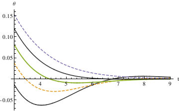
The first method defined - 0.035 < θ < 0.035 as the stop interval. By plotting different functions of θ with different alpha values (0.6, 0.7, 0.8, 0.9, 1.0) in one graph, you can see that α = 0.7 starts to be in the range [-0.035, 0.035] the fastest.

numsola1 =
  NDSolve[{y''[x] == -0.6*2*y'[x] - Sin[y[x]], y[0] == 0.7, y'[0] == 0}, y[x], {x, 0, 1000}]
numsolb1 =
  NDSolve[{y''[x] == -0.7*2*y'[x] - Sin[y[x]], y[0] == 0.7, y'[0] == 0}, y[x], {x, 0, 1000}]
numsolc1 =
  NDSolve[{y''[x] == -0.8*2*y'[x] - Sin[y[x]], y[0] == 0.7, y'[0] == 0}, y[x], {x, 0, 1000}]
numsold1 =
  NDSolve[{y''[x] == -0.9*2*y'[x] - Sin[y[x]], y[0] == 0.7, y'[0] == 0}, y[x], {x, 0, 1000}]
numsolf1 =
  NDSolve[{y''[x] == -1.0*2*y'[x] - Sin[y[x]], y[0] == 0.7, y'[0] == 0}, y[x], {x, 0, 1000}]

Plot[Evaluate[ y[x] /. {numsola1, numsolb1, numsolc1, numsold1, numsolf1}], {x, 3, 9}, PlotStyle -> {GrayLevel[0.2], Dashed, Thick}, PlotRange -> All, AxesLabel -> {"t", "\[Theta]"}, PlotLegends -> {"\[Alpha]=0.6", "\[Alpha]=0.7", "\[Alpha]=0.8", "\[Alpha]=0.9", "\[Alpha]=1.0"}]

To find out more accurate value of α, plot several different α values close to 0.7:

numsola =
  NDSolve[{y''[x] == -0.74*2*y'[x] - Sin[y[x]], y[0] == 0.7, y'[0] == 0}, y[x], {x, 0, 1000}]
numsolb =
  NDSolve[{y''[x] == -0.73*2*y'[x] - Sin[y[x]], y[0] == 0.7, y'[0] == 0}, y[x], {x, 0, 1000}]
numsolc =
  NDSolve[{y''[x] == -0.72*2*y'[x] - Sin[y[x]], y[0] == 0.7, y'[0] == 0}, y[x], {x, 0, 1000}]
numsold =
  NDSolve[{y''[x] == -0.71*2*y'[x] - Sin[y[x]], y[0] == 0.7, y'[0] == 0}, y[x], {x, 0, 1000}]
numsolf =
  NDSolve[{y''[x] == -0.70*2*y'[x] - Sin[y[x]], y[0] == 0.7, y'[0] == 0}, y[x], {x, 0, 1000}]
numsolg =
  NDSolve[{y''[x] == -0.69*2*y'[x] - Sin[y[x]], y[0] == 0.7, y'[0] == 0}, y[x], {x, 0, 1000}]
numsolh =
  NDSolve[{y''[x] == -0.68*2*y'[x] - Sin[y[x]], y[0] == 0.7, y'[0] == 0}, y[x], {x, 0, 1000}]
numsoli =
  NDSolve[{y''[x] == -0.67*2*y'[x] - Sin[y[x]], y[0] == 0.7, y'[0] == 0}, y[x], {x, 0, 1000}]

Plot[Evaluate[ y[x] /. {numsola, numsolb, numsolc, numsold, numsolf, numsolg, numsolh, numsoli}], {x, 3, 8}, PlotStyle -> {GrayLevel[0.1], Dashed, Thick}, PlotRange -> All, AxesLabel -> {"t", "\[Theta]"}, PlotLegends -> {"\[Alpha]=0.74", "\[Alpha]=0.73", "\[Alpha]=0.72", "\[Alpha]=0.71", "\[Alpha]=0.70", "\[Alpha]=0.69", "\[Alpha]=0.68", "\[Alpha]=0.67"}]

Then α = 0.69 should roughly be the critical damping value.

Pi/2*0.005

Out[25]= 0.00785398

findmid[x_, y_] := (x + y)/2

Plot[{DampedDrivenPendulumFunction2[{0.7, 0}, 1, 0, 100][x], DampedDrivenPendulumFunction2[{0.7, 0}, 0.7, 0, 100][x]}, {x, 0, 30}, PlotLegends -> "Expressions", PlotRange -> {-0.007853981633974483`, 0.007853981633974483`}, PlotStyle -> {Thick, Automatic, Dashed}, AspectRatio -> 1.0]

From this graph, when α = 1, the pendulum settles in the stop range faster than when α = 0.7. This means that 0.7 is too small, and 1 may be too large. Then try the mid-value 0.75.

findmid[1, 0.7]

Plot[{DampedDrivenPendulumFunction2[{0.7, 0}, 0.85, 0, 100][x], DampedDrivenPendulumFunction2[{0.7, 0}, 1, 2, 100][x], DampedDrivenPendulumFunction2[{0.7, 0}, 0.7, 0, 100][x]}, {x, 0, 30}, PlotLegends -> "Expressions", PlotRange -> {-0.007853981633974483`, 0.007853981633974483`}, PlotStyle -> {Thick, Automatic, Dashed}, AspectRatio -> 1.0]

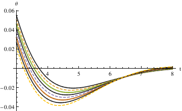
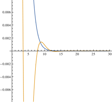
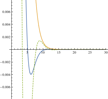
When α = 0.85, the pendulum settles in the range faster than when α = 1. So the critical value may be smaller than 0.85. Try the mid value of 0.85 and 0.7. Finally, the answer yielded from this method is 0.81.

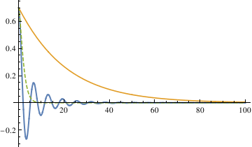
The third method defines the stop interval as not passing 0 in the time span 0 < t \ < 500, uses a function piano to check if the pendulum oscillates.

\[CurlyEpsilon] = 0; g = 9.8;
\[CapitalOmega]0 = 1;
listofsolutions = {};
listofvaluesfor\[Alpha] = Range[0, 2, .0005];
pendulumeq = \[Theta]''[t] + 2*\[Alpha]*\[Theta]'[t] + \[CurlyEpsilon]* Sign[\[Theta]'[t]]*((\[Theta]'[t])^2) + (\[CapitalOmega]0^2)* Sin[\[Theta][t]] == 0;

counter = 1;

While[counter <= Length[listofvaluesfor\[Alpha]], AppendTo[listofsolutions, NDSolve[{Evaluate[ pendulumeq /. {\[Alpha] -> listofvaluesfor\[Alpha][[counter]]}], \[Theta][ 0] == .7, \[Theta]'[0] == 0}, \[Theta][t], {t, 0, 1000}]]; counter++];

evaluatedlistofsolutions = Evaluate[\[Theta][t] /. listofsolutions];

piano is a function that checks to see if the pendulum ever swings past θ = 0 for each of the functions in the list. If the answer is no, then it means that the pendulum no longer oscillates for that value of α.

piano[key_] :=
  Catch[If[FindMinValue[ evaluatedlistofsolutions[[key]], {t, 0, 500}] > 0, Throw[key], Throw[906]]];

counter2 = 1;

While[piano[counter2] == 906, counter2++];

Print["The Value of \[Alpha] at which the function \[Theta][t] stops \ oscillating is ", listofvaluesfor\[Alpha][[counter2]]]

The Value of α at which the function θ[t] stops oscillating is 0.8985

Plot[evaluatedlistofsolutions[[piano[counter2]]], {t, 0, 20}, PlotRange -> All]

Now we assume that α is not zero.

DampedDrivenPendulumFunction2[{\[Theta]0_, \[Omega]0_}, \[Alpha]_, \ \[Epsilon]_, tmax_] :=
  Module[{\[Theta]}, \[Theta] /. First[ NDSolve[{ \[Theta]''[t] == -Sin[\[Theta][t]] - 2 \[Alpha] \[Theta]'[ t] - \[Epsilon] Sign[\[Theta]'[t]] (\[Theta]'[t])^2, \[Theta][0] == \[Theta]0, \[Theta]'[0] == \[Omega]0}, \[Theta], {t, 0, tmax}] ]]

g5 = DampedDrivenPendulumFunction2[{0.7, 0}, 0.1, 1, 100]

g6 = DampedDrivenPendulumFunction2[{0.7, 0}, 10, 1, 100]

g7 = DampedDrivenPendulumFunction2[{0.7, 0}, 1, 1, 100]

Plot[{g5[x], g6[x], g7[x]}, {x, 0, 100}, PlotLegends -> "Expressions", PlotRange -> Full, PlotStyle -> {Thick, Automatic, Dashed}]

When ε is 1, the qualitative difference among different alpha when α is 1, 0.1, or 10 is the same. But when α is 0.1, it oscillates with less times compared to the case when ε is 0.

III. A Real Pendulum

 A real pendulum bob has a finite size and the suspension wire has a mass. In addition, the wire connections to the bob and the support may have some structure. Normally, pendulum osccilations take place in air. All such effects should be taking into account in physical pendulum equation.

 By friction (Coulomb damping). Here \( \quad \omega_0 = \left( g/\ell \right)^{1/2} ,\) and \( \mbox{sign}(x) = \begin{cases} 1, & \ x>0, \\ -1, & \ x<0. \end{cases} \)

Analysis of the experimental data gives the following values of the parameters (Robert A. Nelson and M.G. Olsson, "The pendulum---rich physics from a simple system," American Journal of Physics, Vol. 54, No 2, 112--121, 1986):

 By Archimedes' principle, the apparent weight of the bob is reduced by the weight of the displaced air. This property has the effect of increasing the period since the effective gravity is decreasing. The kinetic energy of the system is partly effected by the air by adding mass to the bob's inertia (but not weight) proportional to the mass of the displaced air. The need for the added mass correction was noted by Friedrich Bessel (1784--1846) in 1828. (It was discovered independently by Pierre Du Buat (1734--1809) in 1786, but only Bessel's work attracted attention to his result.) The dependence of added mass on viscosity was derived by George Stokes (1819--1903) in 1859.

 The length of the pendulum is increased by stretching of the wire due to the weight of the bob. The effective spring constant for a wire of rest length \( \ell_0 \) is

 There is also dynamic stretching of the wire from the apparent centrifugal and Coriolis forces acting on the bob during motion. The corresponding mathematical model leads to a system of differential equations, which is a topic of the second course. See M.G. Olson, American Journal of Physics, Vol. 44, 1211, 1976.

Return to Mathematica page
Return to the main page (APMA0330)
Return to the Part 1 (Plotting)
Return to the Part 2 (First Order ODEs)
Return to the Part 3 (Numerical Methods)
Return to the Part 4 (Second and Higher Order ODEs)
Return to the Part 5 (Series and Recurrences)
Return to the Part 6 (Laplace Transform)
Return to the Part 7 (Boundary Value Problems)