Return to computing page for the first course APMA0330
Return to computing page for the second course APMA0340
Return to computing page for the fourth course APMA0360
Return to Mathematica tutorial for the first course APMA0330
Return to Mathematica tutorial for the second course APMA0340
Return to Mathematica tutorial for the fourth course APMA0360
Return to the main page for the course APMA0330
Return to the main page for the course APMA0340
Return to the main page for the course APMA0360
Return to Part V of the course APMA0330

Preface


This secton provides a stream of examples demonstating applications of power series method for solving initial value problems for second order differential equations.

Examples for second order linear ODEs


Most differential equations can't be solved explicitly in terms of finite combinations of simple familiar functions. Power series solutions, though, are frequently used to obtain recursion equations for the coefficients (of any solution that might be analytic within a neighborhood of the point of expansion). It would be nice, then, to have a function that outputs these equations (given a differential operator as input), rather than just obtaining an approximate solution with a limited radius of accuracy.

As illustration, we present some examples of second order differential equations and show how their solutions could be obtained via power series. It should be noted that power series were historically first used to obtain solutions to initial value problems in 18 and 19 centuries. Now we know some other approximations.

Mathematica is a very powerful package that can be successfully used to determined series solutions of nonlinear differential equations. The following subroutine could be used in this matter.

Clear[seriesDSolve];
seriesDSolve[ode_, y_, iter : {x_, x0_, n_}, ics_: {}] :=
Module[{dorder, coeff},
dorder = Max[0, Cases[ode, Derivative[m_][y][x] :> m, Infinity]];
(coeff =
Fold[Flatten[{#1,
Solve[#2 == 0 /. #1,
Union@Cases[#2 /. #1, Derivative[m_][y][x0] /; m >= dorder,
Infinity]]}] &, ics,
Table[SeriesCoefficient[
ode /. Equal -> Subtract, {x, x0, k}], {k, 0, Max[n - dorder, 0]}]];
Series[y[x], iter] /. coeff) /; dorder > 0]
Then we apply the above subroutine to find a couple of first terms in the series solution:
Clear[seriesDSolve];
seriesDSolve[ y''[x] + x*y'[x] + y[x] == 0, y, {x, 0, 3}, {y[0] -> a, y'[0] -> b}
(*symbolic initial values*)]
SeriesData[x, 0, {a, b, Rational[-1, 2] a, Rational[-1, 3] b}, 0, 4, 1]
The latest version of Mathematica contains a special command: AsymptoticDSolveValue to determine a series solution to linear or quasilinear differential equations.

Example: Consider the initial value problem for the second order differential equation:

\[ y'' +x\,y' + y =0, \qquad y(0) =1, \quad y' (0) =2 . \]
First, we ask Mathematica for determine, say first 15 terms:
ivp = {y''[x] + x*y'[x] + y[x] == 0, y'[0] == 2, y[0] == 1};
Series[DifferentialRoot[Function @@ {{y, x}, ivp}][x], {x, 0, 15}]
Out[2]= 1 + 2 x - x^2/2 - (2 x^3)/3 + x^4/8 + (2 x^5)/15 - x^6/48 - ( 2 x^7)/105 + x^8/384 + (2 x^9)/945 -
x^10/3840 - ( 2 x^11)/10395 + x^12/46080 + (2 x^13)/135135 - x^14/645120 - ( 2 x^15)/2027025 + SeriesData[x, 0, {}, 0, 16, 1]
One may want to separate differential operator from the initial conditions:
ode = y''[x] + x*y'[x] + y[x] == 0;
initconds = {y'[0] == 2, y[0] == 1};
Then we build a differentail operator to create this ode
odeOperator = D[#, {x, 2}] + x*D[#, x] + 1 &;
Now set up our Taylor series as a symbolic expansion using derivatives of y evaluated at the origin. You may want to use an order of 15 but that is something one would probably make as an argument to a function, if automating all this.
yy = Series[y[x], {x, 0, 15}];
Next apply the differential operator and add the initial conditions. Then find a solution that makes all powers of x vanish.
soln = SolveAlways[Join[{odeOperator[yy] == 0}, initconds], x];
Let's look at the Taylor polynomial:
truncatedSol = Normal[yy /. soln[[1]]]
Out[9]= 1 + 2 x - x^2/2 - x^3/3 + x^4/12 + x^5/20 - x^6/90 - x^7/168 + \ x^8/840 + x^9/1728 -
x^10/9450 - x^11/21120 + x^12/124740 + \ x^13/299520 - x^14/1891890 - x^15/4838400
To assess how accurate it might be I will compare with NDSolve
approxSol = NDSolve[Join[{ode}, initconds], y[x], {x, 0, 4}];
Plot[{truncatedSol, y[x] /. approxSol[[1]]}, {x, 0, 4}, PlotLegends -> "Expressions"]
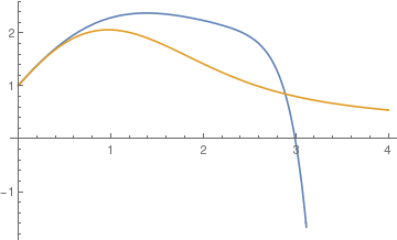
As you see,these two solutions match on the interval [0,0.5], but then diverge from each other. Moreover, the series solution approached minus infinity for x > 3.
AsymptoticDSolveValue[{y''[x] + x*y'[x] + y[x] == 0, y'[0] == 2, y[0] == 1}, y[x], {x, 0, 10}]


Now we consider nonhomogeneous equation \[ x^2 y'' + x\, y' - y = x^2 , \qquad y(1) = \frac{4}{3}, \quad y' (1) = \frac{5}{3} . \] Its solution is \( \displaystyle y(x) = x + \frac{x^2}{3} . \)    ■

Example: The Gross–Pitaevskii equation (GPE, named after Eugene P. Gross and Lev Petrovich Pitaevskii) describes the ground state of a quantum system of identical bosons using the Hartree–Fock approximation and the pseudopotential interaction model. Its stationary model that describes, for example, localization of an atomic gas in trapped Bose--Einstein condensates is

\[ - \frac{{\text d}^2 y}{{\text d}t^2} + \left( 1 - \frac{3}{\cosh^2 (t)} \right) + y^3 =0 , \qquad y(0) =1, \quad y'(0) =0. \]
Its true solution is y(t) = sech t.

The first four Adomian polyniomials are

\begin{align*} A_0 &= u_0^3 , \\ A_1 &= 3\, u_0^2 u_1 , \\ A_2 &= 3\,u_0 u_1^2 + 3\,u_0^2 u_2 , \\ A_3 &= 3\,u_3 u_0^2 + 6\,u_0 u_1 u_2 + u_1^3 . \end{align*}
In general, the Adomian polynomail is a double convolution:
\[ A_m = \sum_{k=0}^m \sum_{j=0}^{m-k} u_k u_j u_{m-k-j} , \qquad m=0,1,2,\ldots . \]
Integrating twice the given differential equation and taking into account the initial conditions, we get
\[ u_{n+1} (t) = \int_0^t {\text d}\tau \int_0^{\tau} \left( \left[ 1 - \frac{3}{\mbox{cosh}^2 (s)} \right] u_n (s) + A_n \left( u)9 *s), \ldots , u_n (s) \right) \right) {\text d}s , \qquad n=0,1,2,\ldots , \]
starting with u0 = 1.    ■

Example: We derive the series solution of the simple pendulum equation, subject to the given initial conditions, up to the order, say, O(t10), for example.

\[ \ddot{x} + \sin (x) =0, \qquad x(0) = \pi /3, \quad \dot{x}(0) = -1/10. \]
Here dot indicate drivative with respect to time variable: \( \texttt{D}x = {\text d}x/{\text d}t = \dot{x} . \) We begin expanding x(t) in a series about t = 0, keeping terms out to order t9. the initial conditions are substituted into the series, the label s being assigned to the result.
s = Series[x[t], {t, 0, 9}] /. {x[0] -> Pi/3, x'[0] -> -1/10}
SeriesData[t, 0, {Rational[1, 3] Pi, Rational[-1, 10], Rational[1, 2] Derivative[2][x][0], Rational[1, 6] Derivative[3][x][0], Rational[1, 24] Derivative[4][x][0], Rational[1, 120] Derivative[5][x][0], Rational[1, 720] Derivative[6][x][0], Rational[1, 5040] Derivative[7][x][0], Rational[1, 40320] Derivative[8][x][0], Rational[1, 362880] Derivative[9][x][0]}, 0, 10, 1]
The simple pendulum equation is entered, the series being automatically substituted and terms grouped according to powers of t.
ode = D[s, {t, 2}] + Sin[s] == 0
For arbitrary time t, the only way that the above output relation can be true is if the coefficient of each power of t is separately set equal to zero. This way be implemented by applying the LogicalExpand command to ode.
eqs = LogicalExpand[ode]
The symbol && appearing between each equation in the output indicates the logical "and". That is to say, the first equation must hold, "and" the second equation, "and" the third, and so on. The equations eqs are then solved for each derivative.
Solve[eqs]
The series solution then follows by replacing derivatives at the initial point in s with the above values.
sol = s /. %[[1]]
Cutting off the asymptotic symbol
Normal[sol]
we obtain the poer series approximation up to the order t9:
\[ x(t) = \frac{\pi}{3} - \frac{t}{10} - \frac{\sqrt{3}}{4}\, t^2 + \frac{t^3}{120} + \frac{17\sqrt{3}}{1600}\, t^4 + \frac{133\,t^5}{80 000} + \frac{2161\sqrt{3}}{1 600 000}\, t^6 - \frac{27 411\, t^7}{112 000 000} - \frac{1 397 461\sqrt{3}}{8 960 000 000}\, t^8 - \frac{10 361 489}{806 400 000 000}\, t^9 . \]
   ■

Example: Consider a simple pendulum problem when its pivot is undergoing vertical oscillations given by A sin(ωt) as in simple pendulum section. Its motion is modeled by the following second order differential equation:

\[ \ddot{\theta} + \frac{1}{\ell} \left[ g - A\,\omega^2 \sin )\omega t) \right] \sin \theta = 0 . \]
Assuming that initial conditions are given
\[ \theta (0) = a , \qquad \dot{\theta} (0) = b , \]
we solve the obtained initial value problem using power series method to obtain
\begin{align*} \theta (t) &= a + bt - \frac{g}{2\ell}\,\sin (a) \,t^2 + \frac{1}{6\ell} \left( A \omega^3 \sin (a) - g\,\cos (a)\,b \right) t^3 + \frac{1}{24\,\ell^2} \left[ 2A\omega^3 \cos (a)\,b\ell + \ell\,\sin (a) \, b^2 g + \sin (a)\,\cos (a)\, g^2 \right] t^4 \\ &\quad - \frac{1}{120\,\ell^2} \left[ 3A\ell\, \sin (a) b^2 \omega^3 + A\omega^5 \ell\,\sin (a) + 4A\,\sin (a)\,\cos (a)\,g\omega^3 - \ell\,\cos (a) \,b^3 g + 3g^2 \sin^2 (a) b - \cos^2 (a) \,bg^2 \right] t^5 \\ &\quad + \frac{1}{720\,\ell^3} \left[ (4\,A^2 \ell \,\sin (a)\,\cos (a) \,\omega^6 - 4\,A\.\ell^2 \cos (a) \, b^3 \omega^3 - 4\,A\,\omega^5 \cos (a) \,b\ell^2 + 16A\,\ell \,\sin^2 (a)\,bg\,\omega^3 - 6A\,\ell \,\cos^2 (a)\, bg\,\omega^3 - \ell^2 \,\sin (a) \,b^4 g - 11\ell\,\sin (a)\,\cos (a)\, b^2 g^2 + 3\,\sin^3 (a) \,g^3 - \sin(a)\.\cos^2 (a) \,g^3 \right] t^6 \\ &\quad - \frac{1}{5040\,\ell^3} \left[ 20\,A^2 \,\ell\,\sin^2 (a) \,b\omega^6 - 10\,A^2 \ell\,\cos^2 (a) \,b\omega^6 - 5\,A*\ell^2 \,\sin (a) \,b^4 \omega^3 - 10\,A\,\ell^2 \sin (a) \,b^2 \omega^5 - A\,\omega^7\, \sin (a)\, \ell^2 - 78\,A\,\ell \, \sin (a) \,\cos (a) \,b^2 g\omega^3 - 11\,A\,\ell\,\sin (a)\,\cos (a) \,g\omega^5 + 25\,A\,\sin^3 (a) \,g^2 \omega^3 - 9\,A\,\sin (a)\,\cos^2 (a) \, g^2\omega^3 + \ell^2 \,\cos (a) \,b^5 g - 15\,\ell\,\sin^2 (a) \,b^3 g^2 + 11\,\ell\,\cos^2 (a) \,b^3 g^2 - 33\,\sin^2 (a)\,\cos (a) \,bg^3 + \cos^3 (a) \,b g^3 \right] t^7 \\ - \frac{1}{40320\,\ell^4} \left[ 138\,A^2 \,\ell^2 \,\sin (a)\.\cos (a) \, b^2 \omega^6 +26 \,A^2 \.\ell^2 \,\sin (a) \,\cos (a) \,\omega^8 - 70\,A^2 \ell\,\sin^3 (a) \,g\omega^6 + 28\,A^2 \ell\,\sin (a) \,\cos^2 (a) \,g\,\omega^6 - 6\,A\,\ell^3 \,\cos (a) \,b^5 \omega^3 - 20\,A\,\ell^3 \,\cos (a) \,b^3 \omega^5 - 6\,A\omega^7 \,\cos (a)\,b\,\ell^3 + 128\,A\,\ell^2 \,\sin^2 (a) \,b^3 g\omega^3 + 66\,A\,\ell^2 \,\sin^2 (a) \,b g\omega^5 - 100\,A\,\ell^2 \,\cos^2 (a) \,b^3 g \omega^3 - 24\,A\,\ell^2 \,\cos^2 (a) \,b g \omega^5 + 348\,A\,\ell\,\sin^2 (a) \,\cos (a) \,b g^2 \omega^3 - 12\,A\,\ell\,\cos^3 (a) \,b g^2 \omega^3 - g\,\ell^3 \,\sin (a) \,b^6 - 57\,\ell^2 \,\sin (a)\,\cos (a) \,b^4 g^2 + 78\,g^3 \,\sin^3 (a) \,b^2 \ell - 102\,\ell\,\sin (a) \,\cos^2 (a) \,b^2 g^3 + 33\,\sin^3 (a) \,\cos (a) \,g^4 - \sin (a) \,\cos^3 (a) \,g^4 \right] t^8 + \cdots . \end{align*}
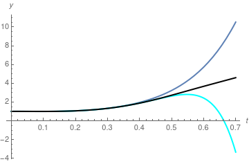
Now we plot two polynomial approximations with n=5 and n=9 terms and compare them with the solution.
a = 1; b = 0.1; L = 1; A = 2.2; omega = 4.4; g = 9.81;
p1[t_] = a + b*t;
p2[t_] = p1[t] - 1/2*g*Sin[a]*t^2/L ;
p3[t_] = p2[t] + 1/6*(A*omega^3*Sin[a] - g*Cos[a]*b)*t^3/L
p4[t_] = p3[t] + 1/24*(2*A*omega^3*Cos[a]*b*L + L*Sin[a]*b^2*g + Sin[a]*Cos[a]*g^2)* t^4/L^2 ;
p5[t_] = p4[t] - 1/120*(3*A*L*Sin[a]*b^2*omega^3 + A*omega^5*Sin[a]*L + 4*A*Sin[a]*Cos[a]*g*omega^3 - L*Cos[a]*b^3*g + 3*g^2*Sin[a]^2*b - Cos[a]^2*b*g^2)*t^5/L^2

p6[t_]= p5[t] + 1/720 (4 A^2 L Sin[a] Cos[a] omega^6 - 4 A L^2 Cos[a] b^3 omega^3 - 4 A omega^5 Cos[a] b L^2 + 16 A L (Sin[a])^2 b g omega^3 - 6 A L (Cos[a])^2 b g omega^3 - L^2 Sin[a] b^4 g - 11 L Sin[a] Cos[a] b^2 g^2 + 3 (Sin[a])^3 g^3 - Sin[a] (Cos[a])^2 g^3)/(L^3) t^6

p7[t_] = p6[t] - 1/5040 (20 A^2 L (Sin[a])^2 b omega^6 - 10 A^2 L (Cos[a])^2 b omega^6 - 5 A L^2 Sin[a] b^4 omega^3 - 10 A L^2 Sin[a] b^2 omega^5 - A omega^7 Sin[a] L^2 - 78 A L Sin[a] Cos[a] b^2 g omega^3 - 11 A L Sin[a] Cos[a] g omega^5 + 25 A (Sin[a])^3 g^2 omega^3 - 9 A Sin[a] (Cos[a])^2 g^2 omega^3 + L^2 Cos[a] b^5 g - 15 L (Sin[a])^2 b^3 g^2 + 11 L (Cos[a])^2 b^3 g^2 - 33 (Sin[a])^2 Cos[a] b g^3 + (Cos[a])^3 b g^3)/(L^3) t^7

p8[t_] = p7[t] - 1/40320 (138 A^2 L^2 Sin[a] Cos[a] b^2 omega^6 + 26 A^2 L^2 Sin[a] Cos[a] omega^8 - 70 A^2 L (Sin[a])^3 g omega^6 + 28 A^2 L Sin[a] (Cos[a])^2 g omega^6 - 6 A L^3 Cos[a] b^5 omega^3 - 20 A L^3 Cos[a] b^3 omega^5 - 6 A omega^7 Cos[a] b L^3 + 128 A L^2 (Sin[a])^2 b^3 g omega^3 + 66 A L^2 (Sin[a])^2 b g omega^5 - 100 A L^2 (Cos[a])^2 b^3 g omega^3 - 24 A L^2 (Cos[a])^2 b g omega^5 + 348 A L (Sin[a])^2 Cos[a] b g^2 omega^3 - 12 A L (Cos[a])^3 b g^2 omega^3 - g Sin[a] b^6 L^3 - 57 L^2 Sin[a] Cos[a] b^4 g^2 + 78 g^3 (Sin[a])^3 b^2 L - 102 L Sin[a] (Cos[a])^2 b^2 g^3 + 33 (Sin[a])^3 Cos[a] g^4 - Sin[a] (Cos[a])^3 g^4)/(L^4) t^8

p9[t_] = p8[t] - 1/362880 (-28 A^3 L Sin[a] (Cos[a])^2 omega^9 + 16 A Sin[a] (Cos[a])^3 g^3 omega^3 - 1238 A^2 L (Sin[a])^2 Cos[a] b g omega^6 + 600 A L^2 Sin[a] Cos[a] b^4 g omega^3 + 444 A L^2 Sin[a] Cos[a] b^2 g omega^5 + 1338 A L Sin[a] (Cos[a])^2 b^2 g^2 omega^3 - 480 A (Sin[a])^3 Cos[a] g^3 omega^3 + 666 L (Sin[a])^2 Cos[a] b^3 g^3 + 52 A^2 L (Cos[a])^3 b g omega^6 - 266 A^2 L^2 (Sin[a])^2 b^3 omega^6 - 182 A^2 L^2 (Sin[a])^2 b omega^8 + 238 A^2 L^2 (Cos[a])^2 b^3 omega^6 + 98 A^2 L^2 (Cos[a])^2 b omega^8 + 7 A L^3 Sin[a] b^6 omega^3 + 35 A L^3 Sin[a] b^4 omega^5 + 21 A L^3 Sin[a] b^2 omega^7 - 126 A L (Sin[a])^3 g^2 omega^5 - 189 (Sin[a])^4 b g^4 + 70 A^3 L (Sin[a])^3 omega^9 + A omega^9 Sin[a] L^3 - L^3 Cos[a] b^7 g + 63 g^2 (Sin[a])^2 b^5 L^2 - 57 L^2 (Cos[a])^2 b^5 g^2 - 102 L (Cos[a])^3 b^3 g^3 + 306 (Sin[a])^2 (Cos[a])^2 b g^4 - (Cos[a])^4 b g^4 + 22 A L^2 Sin[a] Cos[a] g omega^7 - 966 A L (Sin[a])^3 b^2 g^2 omega^3 + 46 A L Sin[a] (Cos[a])^2 g^2 omega^5)/(L^4) t^9 ; Plot[{p6[t], p9[t], Evaluate[y[t] /. sol]}, {t, 0, 0.7`}, PlotRange -> All, PlotStyle -> {{Thick}, {Thick, Cyan}, {Thick, Black}}, Axes -> {True, True}, AxesLabel -> {t, y}]
   ■
  1. Allame, M. and Azad, N., Solution of Third Order Nonlinear Equation by Taylor Series Expansion, World Applied Sciences Journal, 14 (1): 59-62, 2011.


Return to Mathematica page
Return to the main page (APMA0330)
Return to the Part 1 (Plotting)
Return to the Part 2 (First Order ODEs)
Return to the Part 3 (Numerical Methods)
Return to the Part 4 (Second and Higher Order ODEs)
Return to the Part 5 (Series and Recurrences)
Return to the Part 6 (Laplace Transform)
Return to the Part 7 (Boundary Value Problems)