Preface
In the previous section, we show that direction fields or slope fields are very important features of differential equations because they provide a qualitative behavior of solutions. However, more precise information results from including in the plot some typical solution curves or trajectories. It is important to identify other features of the long-term behavior of solutions by including fences, funnels, and separatrix. A plot that shows representative sample of trajectories for a given first order differential equation is called phase portrait. This section shows how to include sample trajectories into tangent field to obtain a phase portrait for a given differential equation.
Return to computing page for the second course APMA0340
Return to Mathematica tutorial for the second course APMA0340
Return to Mathematica tutorial for the fourth course APMA0360
Return to the main page for the course APMA0330
Return to the main page for the course APMA0340
Return to Part II of the course APMA0330
Glossary
Phase portrait
Previously we discussed direction fields that could be visualized by plotting either a list of vectors or lines. However, this information is not detailed on the behavior of specific solutions, as it only shows arrows on a plot indicating the direction of streamlines. The detailed features can only be obtained if we observe the phase portraits. A phase portrait is a graphical tool that consists of some typical solution curves that are needed to determine some other features of streamlines, such as the bounds (or fences), sepatratrix, and other similar properties within varying domains. They are also useful in visualizing the long run behaviors of solutions to differential equations. A helpful way to think of phase portraits is to imagine fish swimming in water with strong currents. Different fish at different positions will have distinct trajectories, and their varying paths can be represented by the lines on a phase portrait.
It can be difficult to give a strict definition of phase portraits because there are no strict, consistent rules for what a phase portrait must contain. The content of a phase portrait will vary depending on the problem or differential equations and the behavior of their solutions. A phase portrait must include enough information to understand the features of the solution and its behavior.
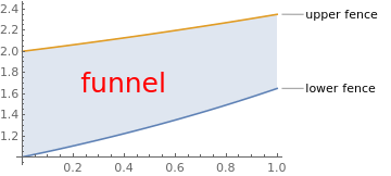
Most differential equations do not have solutions that can be written in elementary form, and even when they do, the search for formulas often obscures the central question: How do solutions behave? One of the ways to trap solution curves is to determine their boundaries---called fences.
txt = Graphics[Text[Style["funnel", Red, Large], {0.4, 1.7}]];
Show[plot, txt]
Correspondingly, Mathematica uses a special command to plot phase portraits: StreamPlot. This command requires a vector-valued input: one for abscissa (usually labeled by
x or t) and another for ordinate. Therefore, to plot a phase portrait for a first order differential
equation \( {\text d}y / {\text d}x = f(x,y) , \) a user needs to set 1 for the first
coordinate and f for the second one, so making the vector input
\( \left( 1, f(x,y) \right) . \) Besides, Mathematica also offers their variations:
ListStreamPlot,
ContourPlot,
ListContourPlot,
ListDensityPlot,
StreamDensityPlot,
ListStreamDensityPlot,
and
LineIntegralConvolutionPlot.
Their applications will be clear from presented examples here. We first start with adding solution curves to the direction fields.
In the previous section, we show how to provide a qualitative information about solution curves to a first order differential equation using direction fields. It is very useful to use Mathematica to graph slope fields, or direction fields. A slope field or tangent fields is a graph that shows a short line segment with slope f(x,y) at every point to the differential equation \( y' = f(x,y) \) in a given range. Plotting such line segments is very tiresome to do by hand, so learning how to do this with a computer algebra system is incredibly useful. In Mathematica, the only one command is needed to draw the direction field corresponding to the equation \( y' =1+t-y^2: \)
dfield = VectorPlot[{1,1+t-y^2}, {t, -2, 2}, {y, -2, 2}, Axes -> True,
VectorScale -> {Small,Automatic,None}, AxesLabel -> {"t", "dydt=1+t-y^2"}]
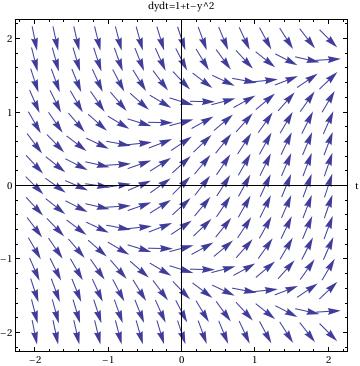
In this command sequence, you enter the VectorPlot command. The first equation gives you the value of {dt,dy} because the slope field graphs dy/dt in this example.
Then you define the ranges for t and y for the graphs.
By commanding the Axes-> True, I am telling Mathematica to put all of the axes on the graph.
The option VectorScale allows one to fix the size of the arrows and Normalize makes the size of the arrows be 1.
The AxesLabel command just labels the two axes on this graph.
Another thing that is very useful to do is to plot the solution to one or more initial value problems on top of the direction field.
To plot the direction field along with, for example, two solutions, we use the following commands:
sol2 = DSolve[{y'[t] == 1 - (y[t])^2 + t, y[0] == -1}, y[t], t]
pp1 = Plot[y[t] /. sol1, {t, -2, 2}]
pp2 = Plot[y[t] /. sol2, {t, -2, 2}]
Show[dfield, pp1, pp2]
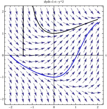
In this command sequence, one first uses DSolve to solve the initial value differential equations. The third and fourth lines tells Mathematica to graph the two solutions to the initial value problem over a set range. The last command, show, tells Mathematica to show both the previously defined direction field, from the last example, and the two solutions to the differential equation. Since I just used an equal sign, =, when this command is entered I will see the solutions to the differential equations on separate graphs and then see a graph that has all three of these components on top of one another.
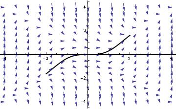
field = VectorPlot[{1, f[x, y]}, {x, -4, 4}, {y, -4, 4}, VectorStyle -> Arrowheads[0.025]]
NDSolve[{y'[x] == f[x, y[x]], y[0] == 0}, y, {x, -2, 2}]
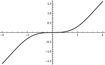
graph = Plot[Evaluate[y[x] /. %], {x, -2, 2}, PlotStyle -> {Black, Thick}]
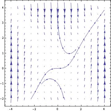
EqnB = DSolve[{y'[x]==x^2 -(y[x])^2, y[0]==-2},y[x],x]
EqnC = DSolve[{y'[x]==x^2 -(y[x])^2, y[0]==2},y[x],x]
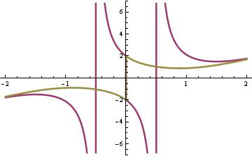
Plot[{Evaluate[y[x]/.EqnA] , Evaluate[y[x]/.EqnB] ,Evaluate[y[x]/.EqnC]},
{x,-2,2},PlotStyle->Thickness[0.007]]
Axes->True, VectorPoints->15, VectorScale->{Tiny,Automatic,None},
StreamPoints ->8, StreamStyle->{Black,"Line"}]
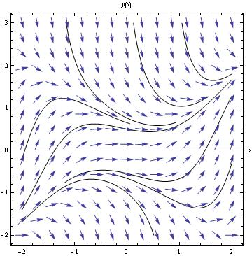
Show[VectorPlot[{1, f[x, y]}, {x, -2, 2}, {y, -2, 8},
VectorStyle -> Arrowheads[0.03]],
Plot[Evaluate[Table[y[x] /. sol, {c, -10, 10, 4}]], {x, -4, 4},
PlotRange -> All]]
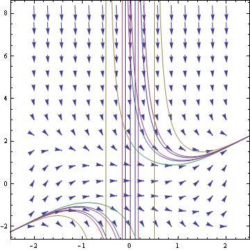
sol = DSolve[y'[x] == f[x, y[x]], y, x] /. C[1] -> c
Show[VectorPlot[{1, f[x, y]}, {x, -2, 2}, {y, -2, 2}, VectorStyle -> Arrowheads[0.026]],
Plot[Evaluate[Table[y[x] /. sol, {c, -10, 10, 1}]], {x, -2, 2}, PlotRange -> All]]
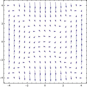
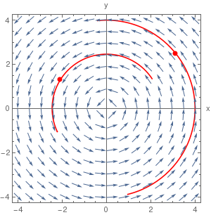
We can a point and a trajectory that goes through this point into a direction field.
Module[{vp},
vp = VectorPlot[{-y, x}, {x, -4, 4}, {y, -4, 4}, VectorScale -> {0.045, 0.9, None}, VectorPoints -> 16];
z = NDSolveValue[
Thread[{x'[t], y'[t], x[0], y[0]} == Join[{-y@t, x@t}, #]], {x@ t, y@t}, {t, -2, 1}] & /@ u;
plot = ParametricPlot[z, {t, -2, 1}, ImageSize -> 300,
Epilog -> {vp[[1]], Red, PointSize[Large], Point[u]},
PlotStyle -> Red, AspectRatio -> 1, Axes -> True,
AxesLabel -> {"x", "y"}, Frame -> True,
PlotRange -> PlotRange[vp]]], {{u, {}}, Locator,
Appearance -> None, LocatorAutoCreate -> All}, {z, {}, None}, {plot, {}, None},
Button["Print snapshot in next cell",
SelectionMove[EvaluationNotebook[], Next, Cell];
NotebookWrite[EvaluationNotebook[], ToBoxes@plot]]]
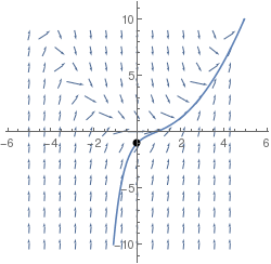
Directon field along with one solution going through a particular point:
plot1 = VectorPlot[{1, f[x, y]}, {x, -5, 5}, {y, -10, 10}, Axes -> True, Frame -> False, VectorScale -> {Tiny, Tiny, None}, ImageSize -> 250];
sol = DSolve[{y'[x] == f[x, y[x]], y[0] == -1}, y[x], x];
ic = y[0] == -1; sol1 = y[x] /. First@DSolve[{y'[x] == x^2 - 2*y[x], ic}, y[x], x]; g[x_] = sol[[1, 1, 2]];
plot2 = Plot[g[x], {x, -5, 5}, PlotRange -> {-10, 10}, ImageSize -> 250];
Show[plot1, plot2, Graphics[{PointSize[Large], Point[{0, -1}]}], ImageSize -> 250]
For plotting streamlines and their solutions, Mathematica has a dedicated command: StreamPlot. Streamlines are similar to vector lines except this command creates lines connecting the different values instead of arrows at each point.
The commands for this function are:
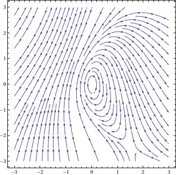
This is a simple command. To use StreamPlot you use almost identical syntax to VectorPlot. The only difference is that for every command in which you use "Vector," you replace this with "Stream." You can also change the aesthetics of the graph in the same manner as VectorPlot.
For plotting streamlines and their solutions, Mathematica has a dedicated command: StreamPlot. Streamlines are similar to vector lines except this command creates lines connecting the different values instead of arrows at each point.
|
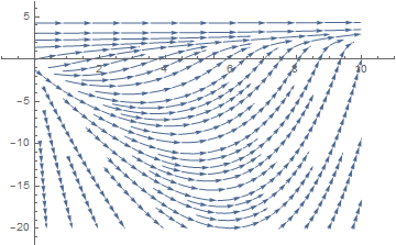
f[x_, y_] = (y + E^(x/2))/(x + E^(2*y))
StreamPlot[{1, f[x, y]}, {x, 0, 10}, {y, -20, 5}, Frame -> False, Axes -> True, AspectRatio -> 1/GoldenRatio] |
 |
|
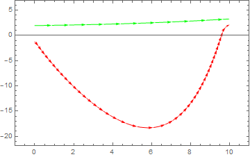
StreamPlot[{1, f[x, y]}, {x, 0, 10}, {y, -20, 5}, Frame -> True,
Axes -> True, AspectRatio -> 1/GoldenRatio,
StreamPoints -> {{{{1, 2}, Green}, {{9.5, -1}, Red}}}] |
 |
|
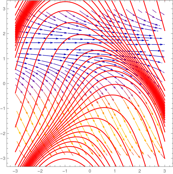
Use numerical solver to plot solutions along with the direction field for the differential equation
\[
y' = \cos (y) -x .
\]
soln[y0_?NumericQ] :=
First@NDSolve[{y'[x] == -x + Cos[y[x]], y[0] == y0}, {y}, {x, -10,
10}];
sp = StreamPlot[{1, (-1 + Sin[y])}, {x, -3, 3}, {y, -3, 3}];
Show[sp,
Plot[Evaluate[{y[x]} /. soln[#] & /@ Range[-20, 20, 0.3]], {x, -3,
3}, PlotRange -> All, MaxRecursion -> 8, AxesLabel -> {"x", "y"},
PlotStyle -> Red]]
|
 |
StreamPlot:
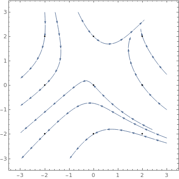
ListStreamPlot
|
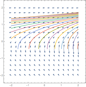
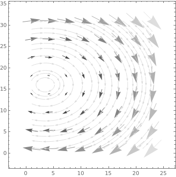
ListStreamPlot[Table[{y, -x}, {x, -.5, 4, 0.2}, {y, -3, 3, 0.2}],
StreamStyle -> LightGray, VectorPoints -> 8, VectorColorFunction -> GrayLevel] |
 |
|
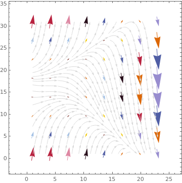
data = Table[{1, y^2 - x^2}, {x, -.5, 4, 0.2}, {y, -3, 3, 0.2}];
ListStreamPlot[data, StreamStyle -> LightGray, VectorPoints -> 8, VectorColorFunction -> Function[{x, y, vx, vy, n}, ColorData[22][Round[n]]], VectorColorFunctionScaling -> False] ListStreamPlot[data, StreamStyle -> LightGray, VectorPoints -> 8, VectorColorFunction -> Function[{x, y, vx, vy, n}, Hue[x, y, 1]], VectorColorFunctionScaling -> {False, True}] |
 |
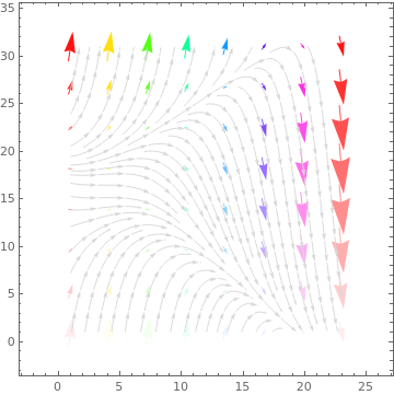 |
|
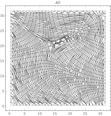
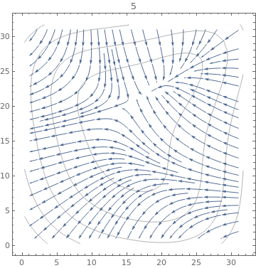
ListStreamPlot[data, StreamStyle -> LightGray, VectorPoints -> 8,
VectorColorFunction -> Function[{x, y, vx, vy, n}, Hue[n, y, 1]], VectorColorFunctionScaling -> {True, True, True, True, False}] |
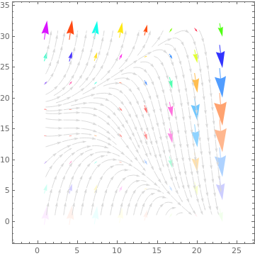 |
 |
 |
 |
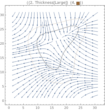 |
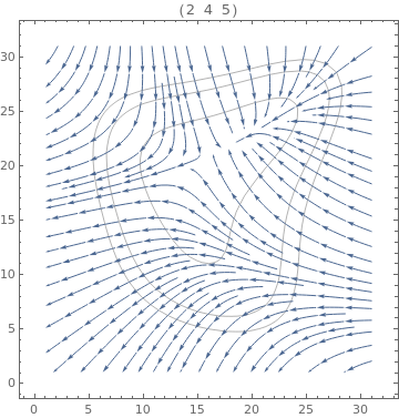
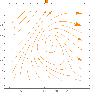
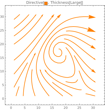
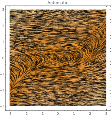
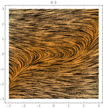
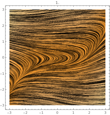
Table[ListStreamPlot[data, StreamPoints -> Coarse, StreamScale -> Full, StreamStyle -> s,
PlotLabel -> s], {s, {Orange, Thick, Directive[Orange, Thick]}}]
 |
 |
 |
ContourPlot
|
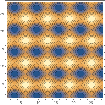
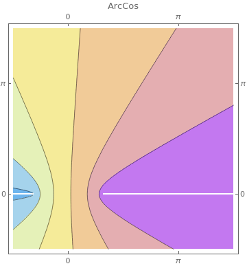
ContourPlot[2 Cos[x] - 3 Sin[y], {x, 1, 9 Pi}, {y, 1, 9 Pi},
PlotLegends -> Automatic]
|
 |
|
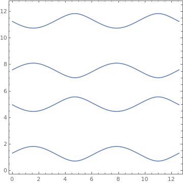
ContourPlot[Sin[x] + 2 Cos[y] == 1/2, {x, 0, 4 Pi}, {y, 0, 4 Pi}]
|
 |
|
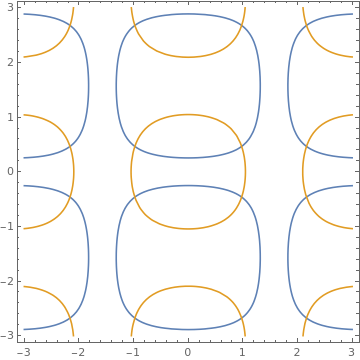
ContourPlot[{Abs[Cos[x] 2*Sin[y]] == 0.5,
Abs[Cos[x] Cos[y]] == 0.5}, {x, -3, 3}, {y, -3, 3}]
|
 |
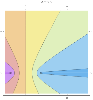
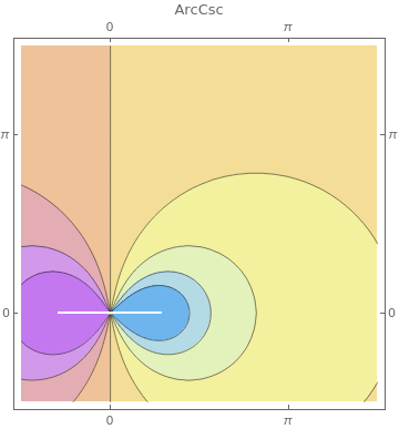
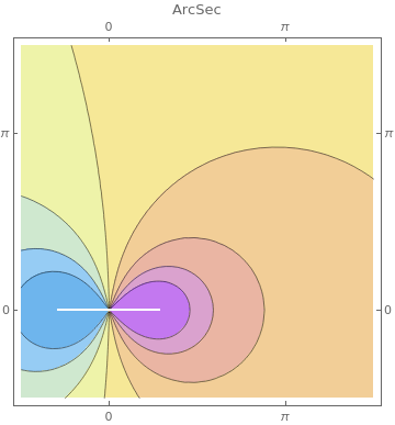
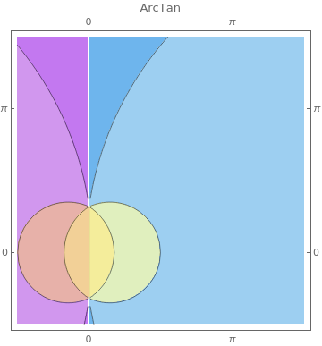
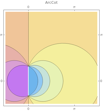
PlotLabel -> f, FrameTicks -> {{-Pi, 0, Pi}, {-Pi, 0, Pi}},
ClippingStyle -> Automatic, ColorFunction -> "Pastel"], {f, {ArcSin, ArcCos, ArcCsc, ArcSec, ArcTan, ArcCot}}]
 |
 |
 |
 |
 |
 |
ListContourPlot
|
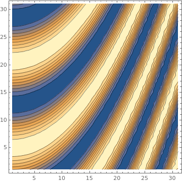
ListContourPlot[
Table[Sin[4 i - 2 j^2], {i, 0, 3, 0.1}, {j, 0, 3, 0.1}]]
|
 |
|
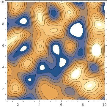
ListContourPlot[RandomReal[10, {10, 10}], InterpolationOrder -> 6,
PlotLegends -> Automatic]
|
 |
|
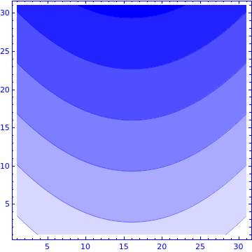
ListContourPlot[
Table[-3 i + j^2, {i, -1.5, 1.5, 0.1}, {j, -1.5, 1.5, 0.1}],
PlotTheme -> {"Monochrome", Blue}]
|
 |
|
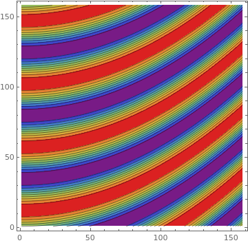
ListContourPlot[
Table[Sin[-j^2 + 7 i], {i, 0, Pi, 0.02}, {j, 0, Pi, 0.02}],
ColorFunction -> "Rainbow", PlotLegends -> Automatic]
|
 |
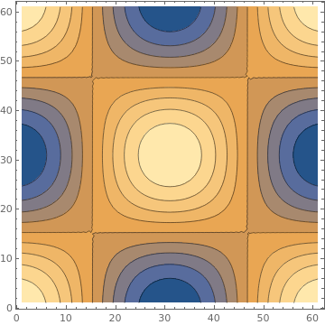
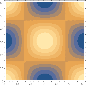
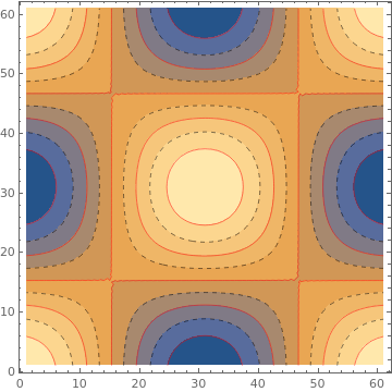
{ListContourPlot[data, ContourStyle -> Black],
ListContourPlot[data, ContourStyle -> None],
ListContourPlot[data, ContourStyle -> {Red, Dashed}]}
 |
 |
 |
ListDensityPlot
|
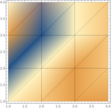
ListDensityPlot[{{3, 2, 1, 1}, {-1, 3, 1, 2}, {1, -1, 3, 2}, {3, 0, 3,
2}}, Mesh -> All]
|
 |
|
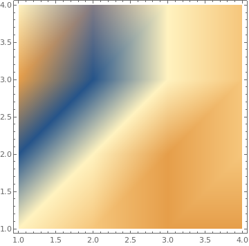
ListDensityPlot[{{3, 2, 1, 1}, {-1, 3, 1, 2}, {1, -1, 3, 2}, {3, 0, 3,
2}}, Mesh -> All]
|
 |
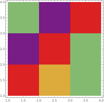
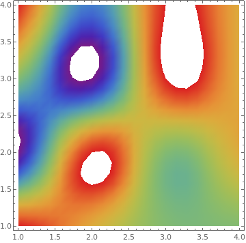
{ListDensityPlot[data, InterpolationOrder -> 0, ColorFunction -> "Rainbow"],
ListDensityPlot[data, InterpolationOrder -> 2, ColorFunction -> "Rainbow"],
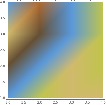
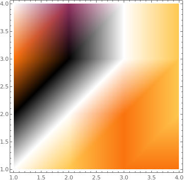
ListDensityPlot[data, InterpolationOrder -> o, ColorFunction -> "SouthwestColors"],
ListDensityPlot[data, InterpolationOrder -> o, ColorFunction -> "SunsetColors"]}
 |
 |
 |
 |
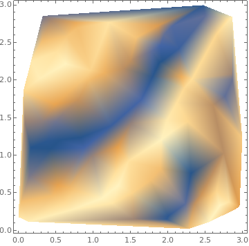
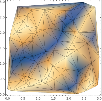
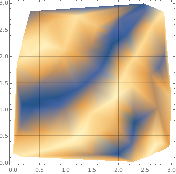
{ListDensityPlot[data, Mesh -> Full], ListDensityPlot[data, Mesh -> All], ListDensityPlot[data, Mesh -> 5]}
 |
 |
 |
|
data = Table[
With[{r = RandomReal[{0, 5}],
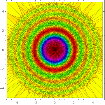
t = RandomReal[{0, 2 Pi}]}, {r Cos[t], r Sin[t], Sin[r^2]/r^2}], {10^4}]; ListDensityPlot[data, InterpolationOrder -> 0, ColorFunction -> Hue, Mesh -> All] |
 |
StreamDensityPlot
ColorFunction -> "ThermometerColors"]
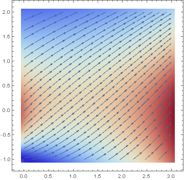
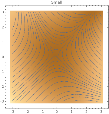
StreamScale -> p, PlotLabel -> p], {p, {Small, Large}}]
 |
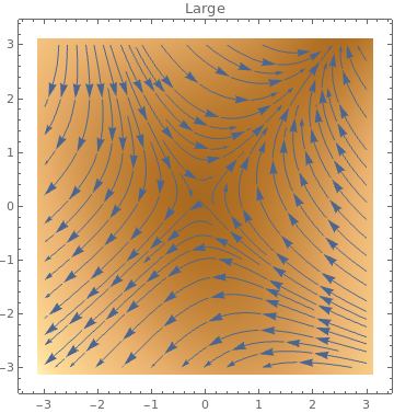 |
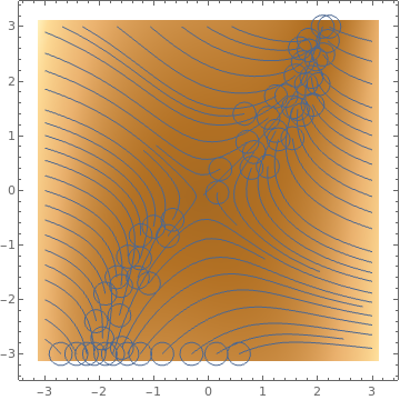
StreamScale->Full,StreamStyle->s],{s,{"Toothpick","Dart",
Directive[Orange,Dashed],Arrowheads[{{0.03,Automatic,Graphics[Circle[]]}}]}}]
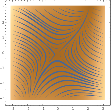 |
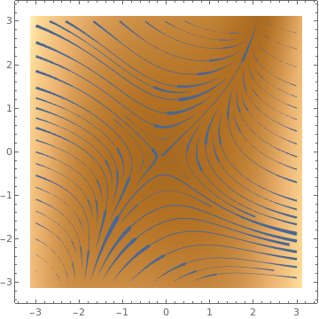 |
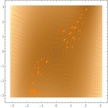 |
 |
ListStreamDensityPlot
|
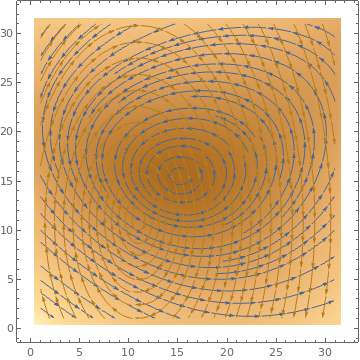
data1 = Table[{-1 + x^2 - 9 y, 1 + 6 x - y^2}, {x, -3, 3, .2}, {y, -3,
3, .2}];
data2 = Table[{2 y, -6 x}, {x, -3, 3, .3}, {y, -3, 3, .3}]; ListStreamDensityPlot[{data1, data2}] |
 |
|
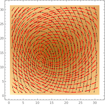
data1 = Table[{-1 + x^2 - 9 y, 1 + 6 x - y^2}, {x, -3, 3, .2}, {y, -3,
3, .2}];
data2 = Table[{2 y, -6 x}, {x, -3, 3, .3}, {y, -3, 3, .3}]; ListStreamDensityPlot[{data1, data2}, StreamStyle -> {{Red, "Drop"}, {Black, "Dart"}}] |
 |
|
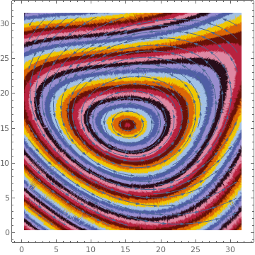
data = Table[{-1 + x^2 - 9 y, 1 + 6 x - y^2}, {x, -3, 3, .2}, {y, -3,
3, .2}];
ListStreamDensityPlot[data, MaxRecursion -> 4, ColorFunctionScaling -> False, ColorFunction -> Function[{x, y, vx, vy, n}, ColorData[22][Round[n]]]] |
 |
|
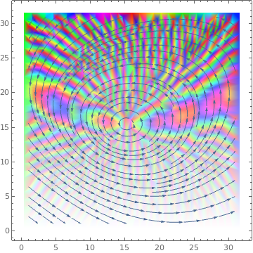
data = Table[{-1 + x^2 - 9 y, 1 + 6 x - y^2}, {x, -3, 3, .2}, {y, -3,
3, .2}];
ListStreamDensityPlot[data, ColorFunctionScaling -> {False, True}, ColorFunction -> Function[{x, y, vx, vy, n}, Hue[x, y, 1]]] |
 |
LineIntegralConvolutionPlot
 |
 |
 |
 |
|
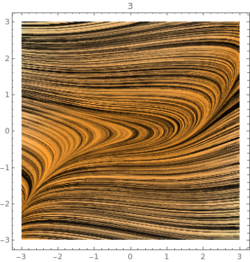
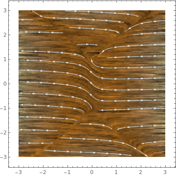
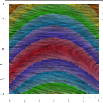
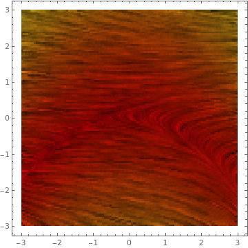
LineIntegralConvolutionPlot[{-1 - 13 x^2 + y^4,
1 - x - .5 y^2},
{x, -3, 3}, {y, -3, 3}, StreamPoints -> Coarse, StreamStyle -> LightBlue] |
 |
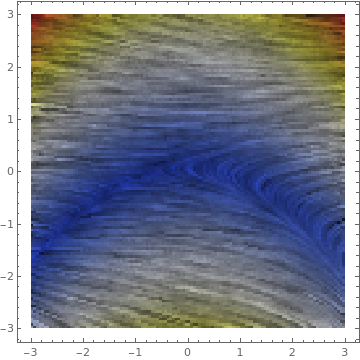
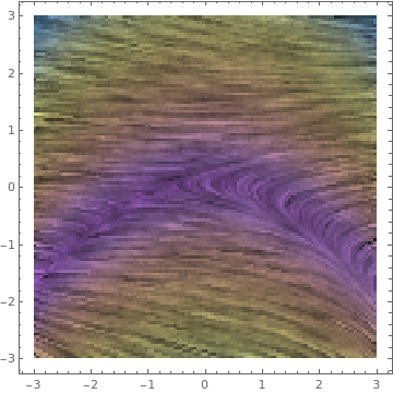
{x, -3, 3}, {y, -3, 3}, ColorFunction -> p],
{p, {"TemperatureMap", "Pastel", "BrightBands", "SolarColors"}}]
 |
 |
 |
 |
|
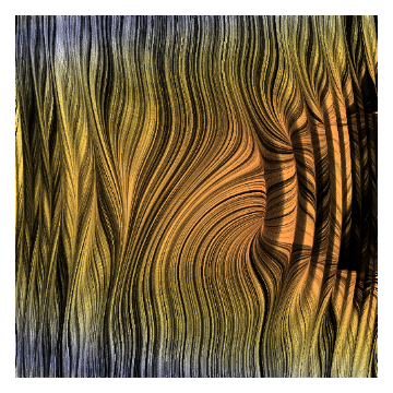
LineIntegralConvolutionPlot[{{Cos[y^2 + x^3], 1 - x + y^2},
{"noise", 500, 500}}, {x, -3, 3}, {y, -3, 3}, ColorFunction -> "BeachColors", LightingAngle -> 0, LineIntegralConvolutionScale -> 3, Frame -> False] |
 |
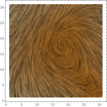
ListLineIntegralConvolutionPlot
ListLineIntegralConvolutionPlot[data]
Return to Mathematica page)
Return to the main page (APMA0330)
Return to the Part 1 (Plotting)
Return to the Part 2 (First Order ODEs)
Return to the Part 3 (Numerical Methods)
Return to the Part 4 (Second and Higher Order ODEs)
Return to the Part 5 (Series and Recurrences)
Return to the Part 6 (Laplace Transform)
Return to the Part 7 (Boundary Value