Preface
This section discusses a simplified version of the Adomian decomposition method first concept of which was proposed by Randolf Rach in 1989 that was crystallized later in a paper published with his colleagues G. Adomian and R.E. Meyers. That is way this technique is frequently referred to as the Rach--Adomian--Meyers modified decomposition method (MDM for short). Initially, this method was applied to power series expansions, which was based on the nonlinear transformation of series by the Adomian--Rach Theorem. Similar to the Runge--Kutta methods, the MDM can be implemented in numerical integration of differential equations by one-step methods. In case of polynomials or power series, it shows the advantage in speed and accuracy of calculations when at each step the Adomian decomposition method allows one to perform explicit evaluations.
Return to computing page for the second course APMA0340
Return to Mathematica tutorial for the second course APMA0340
Return to the main page for the course APMA0330
Return to the main page for the course APMA0340
Return to Part VII of the course APMA0330
Glossary
Falkner--Skan layer
MATHEMATICA TUTORIAL for the First Course. Part VII: Tridiagonal linear systems
Preface
This tutorial was made solely for the purpose of education and it was designed for students taking Applied Math 0330. It is primarily for students who have very little experience or have never used Mathematica and programming before and would like to learn more of the basics for this computer algebra system. As a friendly reminder, don't forget to clear variables in use and/or the kernel. The Mathematica commands in this tutorial are all written in bold black font, while Mathematica output is in normal font.
Finally, you can copy and paste all commands into your Mathematica notebook, change the parameters, and run them because the tutorial is under the terms of the GNU General Public License (GPL). You, as the user, are free to use the scripts for your needs to learn the Mathematica program, and have the right to distribute this tutorial and refer to this tutorial as long as this tutorial is accredited appropriately. The tutorial accompanies the textbook Applied Differential Equations. The Primary Course by Vladimir Dobrushkin, CRC Press, 2015; http://www.crcpress.com/product/isbn/9781439851043
Return to computing page for the second course APMA0340
Return to Mathematica tutorial for the first course APMA0330
Return to Mathematica tutorial for the second course APMA0340
Return to the main page for the course APMA0330
Return to the main page for the course APMA0340
Return to Part VII of the course APMA0330
Glossary
Tridiagonal linear systems
The solution of linear systems of equations is one of the most important areas of computational mathematics. We are not going to present this topic in detail---it deserves a special course. Instead, we consider one particular and very important case when the leading matrix is tridiagonal:

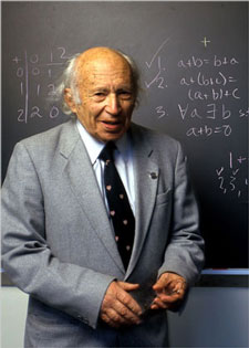
This system of algebraic equations could be solved using standard Gaussian elimination procedure, which actually reduces the problem to an upper triangular form. This stage is usually referred to as the forward elimination (FE). Once it is completed, the second stage, which is called backward substitution (BS), involves finding actual solution. Therefore, this algorithm is usually called FEBS, or in computational jargon "progonka." In engineering, the FEBS method is associated with the British scientist Llewellyn H. Thomas from Bell laboratories who solved a simple Poisson problem (see following example) using this method in 1946. Historically, a prominent Soviet mathematician Israel Moiseevich Gelfand (1913--2009) discovered FEBS algorithm in 1933 being a sophomore college student. He personally refused to associate his name with FEBS because, in his opinion, it was a very simple application of Gaussian elimination. Instead, he suggested to call FEBS algorithm as "progonka (прогонка)," and this slang is widely accepted.
Using the elimination procedure, the augmented matrix is reduced to an equivalent upper triangular form:
FEBS (progonka) algorithm

% elimination stage


for i = 2 to n

	d(i) = d(i) - u(i-1)*l(i)/d(i-1)

	b(i) = b(i) - b(i-1)*l(i)/d(i-1)

endfor


% backward substitution


x(n) = b(n)/d(n)

for i=n-1 downto 1

	x(i) = (b(i) - u(i)*x(i+1))/d(i)

endfor
Theorem: If the tridiagonal matrix A is diagonally dominant (\( d_i > |l_i | + |u_i | > 0, \quad 1 \le i \le n; \) ), then FEBS algorithm will succeed in producing the correct solution to the original linear system, within the limitations of rounding error. ■
Example: Consider the Dirichlet problem on the interval [0,1]:
We divide the interval [0,1] into n equal subintervals \( x_{k-1} , x_k ] , \) according to
Return to Mathematica page
Return to the main page (APMA0330)
Return to the Part 1 (Plotting)
Return to the Part 2 (First Order ODEs)
Return to the Part 3 (Numerical Methods)
Return to the Part 4 (Second and Higher Order ODEs)
Return to the Part 5 (Series and Recurrences)
Return to the Part 6 (Laplace Transform)
Return to the Part 7 (Boundary Value Problems)