We present some applications of differential equations of order greater than one.
Example 1: (Flow Problem)
A 500 liter container initially contains 10 kg of salt. A brine mixture of
100 grams of salt per liter is entering the container at 6 liter per minute.
The well-mixed contents are being discharged from the tank at the rate of
6 liters per minute.
Express the amount
of salt in the container as a function of time.
Salt is coming at the rate: 6*(0.1)=0.6 kg/min
d yin /dt =0.6 ; d yout/dt = 6x/500
dx/dt = 0.6 -6x/500 ; x(0)=10
DSolve[{x'[t]==6/10-6*x[t]/500, x[0]==10},x[t],t]
Out[15]= {{x[t] -> 10 E^(-3 t/250) (-4 + 5 E^(3 t/250))}}
Suppose that the rate of discharge is reduced to 5 liters per minute.
DSolve[{x'[t]==6/10-5*x[t]/(500+t), x[0]==10},x[t],t]
SolRule[t_] = Apart[x[t] /. First[%]]
Out[1]= {{x[t] -> (1/(
10 (500 + t)^5))(3125000000000000 + 187500000000000 t +
937500000000 t^2 + 2500000000 t^3 + 3750000 t^4 + 3000 t^5 + t^6)}}
Out[2]= 50 + t/10 - 1250000000000000/(500 + t)^5
To check the answer:
Simplify[SolRule'[t] == 6/10 - 5*SolRule[t]/(500 + t)]
Together[SolRule'[t] == Together[6/10 - 5*SolRule[t]/(500 + t)]]
SolRule[0]
Out[3]= True
Out[4]= True
Out[5]= 10
■
End of Example 1
Example 2:
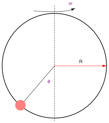
Consider a bead of mass m on a rotating hoop of radius R.
circle = Graphics[{Thick, Circle[{0, 0}, 1]}]
disk = Graphics[{Pink, Disk[{-0.65, -0.75}, 0.1]}]
linev = Graphics[{Dashed, Line[{{0, 1.15}, {0, -1.05}}]}]
line = Graphics[Line[{{0, 0}, {-0.6, -0.7}}]]
ar = Graphics[
Arrow[BezierCurve[{{-0.4, 1.05}, {0.2, 1}, {0.4, 1.1}}]]]
arrow = Graphics[{Red, Arrow[{{0, 0}, {1, 0}}]}]
text1 = Graphics[
Text[Style["\[Theta]", FontSize -> 14, Purple], {-0.11, -0.3}]]
text2 = Graphics[
Text[Style["\[Omega]", FontSize -> 14, Purple], {0.31, 1.2}]]
text3 = Graphics[Text[Style["R", FontSize -> 14, Black], {0.5, 0.08}]]
Show[circle, arrow, ar, line, linev, disk, text1, text2, text3]
disk2 = Graphics[{Pink, Disk[{0.65, -0.75}, 0.1]}];
linev2 = Graphics[{Dashed, Line[{{0, 1.0}, {0, -1.0}}]}];
line2 = Graphics[Line[{{0, 0}, {0.6, -0.7}}]];
tilt = Graphics[{Dashed, Line[{{0.25, 0.97}, {-0.3, -1.2}}]}];
ar2 = Graphics[
Arrow[BezierCurve[{{-0.5, -1.3}, {-0.0, -1.55}, {-0.1, -1.1}}]]];
rAngls = {{0.7, {-11.4*Pi/8, 10.33*Pi/6}}};
directives = {Directive[Red, Thick,
Arrowheads[{{-0.05, 0}, {0.05, 1}}]]};
arcsWArrows[args1 : {{_, {_, _}} ..},
dir_List: {Directive[GrayLevel[.3],
Arrowheads[{{-0.05, 0}, {0.05, 1}}]]}] :=
ParametricPlot[
Evaluate[#[[1]]*{Cos[Rescale[u, {0, 2 Pi}, Abs@#[[2]]]],
Sin[Rescale[u, {0, 2 Pi}, Abs@#[[2]]]]} & /@ args1], {u, 0,
2 Pi}, PlotStyle -> dir, Axes -> False, PlotRangePadding -> .2,
ImageSize -> 200] /. Line[x_, ___] :> Arrow[x]
ar3 = arcsWArrows[rAngls, {directives[[1]]}];
text1 = Graphics[
Text[Style["\[Theta]", FontSize -> 14, Purple], {0.21, -0.80}]];
text2 = Graphics[
Text[Style["\[Omega]", FontSize -> 14, Purple], {0.1, -1.3}]];
text4 = Graphics[
Text[Style["\[Alpha]", FontSize -> 14, Black], {0.1, 0.85}]];
Show[circle, arrow, ar2, line2, linev2, disk2, text1, text2, text3,
text4, tilt, ar3]
|
Schematic representation of the bead-on-a-hoop
|
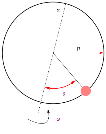
A hoop tilted on angle α
|
The kinetic energy reads
\[
\mbox{K} = \frac{1}{2}\,m R^2 \left( \dot{\theta}^2 + \sin^2 \theta \,\omega^2 \right) .
\]
The potential energy is
\[
\Pi = -mgR \left( \cos\alpha \,\cos \theta + \sin \alpha \,\cos \omega t \,\sin \theta \right) ,
\]
where θ is the angle measured from the bottom of the hoop with respect to the direction of the rotation axis and α is the angle formed between the rotation axis and the vertical direction. If there exist a friction, which could be modeled by the force
\[
{\bf F} = - c{\bf v} ,
\]
which leads to the generalized force
\[
Q = -c R^2 \dot{\theta} \qquad\mbox{since} \quad {\bf v} = R\dot{\theta} .
\]
Inserting these expressions into the Lagrangian
\( L = \mbox{K} - \Pi , \) and applying the Euler--Lagrange equations, we obtain the equation of motion:
\[
\ddot{\theta} + \frac{c}{m}\,\dot{\theta} + \left( \frac{g}{R}\,\cos\alpha - \omega^2 \cos\theta \right) \sin \theta = \frac{g}{R} \,\sin \alpha \,\cos\theta \,\cos \omega t .
\]
If the tilt angle α is small, the above equation can be linearized in α by natural substitution:
\[
\ddot{\theta} + \frac{c}{m}\,\dot{\theta} + \left( \frac{g}{R} - \omega^2 \cos\theta \right) \sin \theta = \frac{g}{R} \, \alpha \,\cos\theta \,\cos \omega t .
\]
If rotation is along vertical axis (α = 0), we get a homogeneous differential equation
\[
\ddot{\theta} + \frac{c}{m}\,\dot{\theta} + \left( \frac{g}{R} - \omega^2 \cos\theta \right) \sin \theta = 0.
\]
The equilibrium positions θ = θ
*, associated to the condition that θ and its velocity are both zeroes, are obtained by solving either
\[
\sin \theta =0 \qquad\mbox{or} \qquad \frac{g}{R} - \omega^2 \cos\theta =0 ,
\]
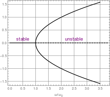
This gives three physical stationary points:
\[
\theta^{\ast} = 0, \quad \pi , \quad \arccos \left( \frac{g}{\omega^2 R} \right) ,
\]
subject to condition
\[
\omega \ge \omega_c = \sqrt{\frac{g}{R}} .
\]
Therefore, if the angular velocity of the hoop ω is greater than a
critical angular velocity ω
c, we observe the third critical point; otherwise thare are only two of them. This situation indicates that we observe a
supercritical pitchfork bifurcation about the stationary value ω
c.
line = Graphics[{Thick, Line[{{0, 0}, {1, 0}}]}];
curve1 = Plot[Sqrt[x - 1], {x, 1, 3.5}, PlotStyle -> {Thick, Black}];
curve2 = Plot[-Sqrt[x - 1], {x, 1, 3.5}, PlotStyle -> {Thick, Black}];
line2 = Graphics[{Thick, Dashed, Line[{{3.8, 0}, {1, 0}}]}];
text1 = Graphics[
Text[Style["stable", FontSize -> 14, Purple], {0.5, 0.1}]];
text2 = Graphics[
Text[Style["unstable", FontSize -> 14, Purple], {2.5, 0.1}]];
Show[text1, text2, line, line2, curve1, curve2,
FrameLabel -> {"\[Omega]/\!\(\*SubscriptBox[\(\[Omega]\), \(c\)]\)",
None}, Frame -> True, GridLines -> Automatic]
Bifurcation diagram
■
End of Example 2
Example 3:
Example: Move to chapter 4, application4
Consider the Lane--Emden type
equation with an exponential nonlinearity of the
solution with respect to the variable base
\[
\frac{{\text d}^2 y}{{\text d}x^2} + \frac{2}{x}\, \frac{{\text d}y}{{\text d}x} + (x+1)^{y(x)}, \qquad y(0) =1, \quad y' (0) =0.
\]
■
End of Example 3
Example 4:
Consider the initial value problem for undamped Duffing equation:
\[
y'' + k\, y =0, \qquad y(0) = \varepsilon \,y^3 , \quad y' (0) =0.
\]
We can rewrite the Duffing equation in the operator form:
\[
L\left[ y \right] \equiv \texttt{D}^2 y = N \left[ y \right] \equiv
\varepsilon \,y^3 - k\, y.
\]
Physically, the resilience of the oscillator is directly proportional to
N[
y]. When
k ≥ 0 and ε < 0, there is one
unique equilibrium point
y = 0 where the nonlinear term vanishes.
However, when
k ≤ 0 and ε > 0, there are two
equilibrium points:
y = 0 and
\( y = \sqrt{|k/\varepsilon |} . \)
From the physical points of view, the sum of the kinetic and
potential energy of the oscillator keeps the same, therefore it is clear that
the oscillation motion is periodic, no matter
k is positive or
negative. Thus, from physical points of view, it is easy to know that
y(
t) is periodic, even if we do not directly solve the Duffing
equation.
■
End of Example 4
Example 5: (Flow Problem)
Our example is based on Gladkov's article. Although the problem of brachistochrone, which was stated by Johann Bernoulli in 1696, has been discussed previously in section on Reduction higher order ODEs, we reconsider this problem when an object slides under the Coulomb friction force.
We assume that an object is spherical form is rolling over a curve without slip under gravity in
vacuum and the sphere is decelerated only by the force
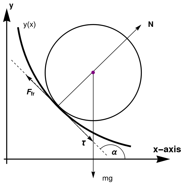
of interaction with the body according to the Coulomb law. A schematic of the forces and geometric statement of the problem are given in the following figure.
15], {-0.16, 1.0}], Black,
Text[Style["mg", FontSize -> 15], {0.65, -0.6}],
Text[Style["x-axis", FontSize -> 18, Bold], {1.27, -0.3}],
Text[Style[Subscript[F, fr], FontSize -> 15, Bold], {-0.15, 0.3}],
Text[Style[\[Tau], FontSize -> 18, Bold], {0.4, -0.23}],
Text[Style["y", FontSize -> 15, Bold], {-0.35, 1.2}],
Text[Style["N", FontSize -> 15, Bold], {1.1, 1.0}],
Text[Style[\[Alpha], FontSize -> 15, Bold], {0.72, -0.33}]}];
Show[curve, circle, line, ar1, ar2, ar3, ar4, arx, ary, dot, angle, \
txt]
Rolling sphere
The equation of motion can
always be written as Newton’s second law:
\[
m\mathbf{a} = \mathbf{F}_{fr} + \mathbf{N} + m\mathbf{g} ,
\tag{5.1}
\]
where
m is the sphere mass,
Ffr is the Coulomb friction
force,
N is the reaction force, and
g is the acceleration of gravity.
The acceleration in curvilinear coordinates is
\[
\mathbf{a} = \dot{v}\,\tau + \frac{v^2}{R}\,\mathbf{n} ,
\]
where
τ − n is the moving basis shown in the figure,
R is the radius of curvature of the motion path,
τ is the unit
vector of the tangent directed along the velocity, and
n
is the normal vector. From here on, a dot above a variable means time differentiation, and it is assumed that
v =
v(
t).
Since
\[
\begin{split}
\mathbf{F}_{fr} &= - F_{fr}\tau , \qquad \mathbf{N} = \mathbf{n}\,N ,
\\
\mathbf{g} &= \left( \tau\,\sin\alpha + \mathbf{n}\,\cos\alpha \right) ,
\end{split}
%\tag{5.2}
\]
where obtuse angle α(
t) belongs to the closed segment [π/2, π]. Eq.(5,1) can be written as
\[
m \left( \dot{v}\,\tau + \frac{v^2}{R} \,\mathbf{n} \right) = - F_{fr} \tau + N\,\mathbf{n} + mg \left( \tay\,\sin\alpha + \mathbf{n}\,\cos\alpha \right) .
\]
Having projected this equation to the basis
τ–
n, we
arrive at the following system of equations:
\[
\begin{cases}
\dot{v} &= g\,\sin\alpha - \frac{1}{m}\, F_{tr} ,
\\
\frac{m\,v^2}{R} &= N + mg\,\cos\alpha .
\end{cases}
\tag{5.2}
\]
It follows from the lower equation that the reaction
force is
\[
N = m \left( \frac{v^2}{R} - g\,\cos\alpha \right) .
\]
When considering brachistochrone, the following
condition should be satisfied (as was demonstrated
in the article by A. A. Barsuk and F. Paladi,
International Journal of Non-Linear Mechanics,
148, 43 (2023).):
\[
\frac{v^2}{R} = -g\,\cos\alpha .
\]
(Note that, if
\( \displaystyle \quad v = g\, \cos\alpha , \quad \) the trajectory is a parabola.) Therefore, according to
\( \displaystyle \quad N = m \left( \frac{v^2}{R} - g\,\cos\alpha \right) , \quad \) the reaction force is
\[
N = -2mg\,\cos\alpha \ge 0 .
\]
Hence, the friction force becomes
\[
F-{gr} = \mu\, N = -2\mu \,mg\,\cos\alpha .
\]
This allows us to rewrite the system of equation (5.2) as
\[
\begin{cases}
\dot{v} &= g\left( \sin\alpha + 2\mu \,\cos\alpha \right) ,
\\
\frac{m\,v^2}{R} &= -g\,\cos\alpha .
\end{cases}
\tag{5.3}
\]
Since
\[
v = R\,\dot{\alpha} ,
\]
we arrive at the following system instead of Eq.(5.3),
which is much simpler:
\[
\begin{cases}
\dot{v} &= g\left( \sin\alpha + 2\mu \,\cos\alpha \right) ,
\\
v],\dot{\alpha} &= -g\,\cos\alpha .
\end{cases}
\tag{5.4}
\]
Having divided the upper equation by the lower, we
obtain
\[
\frac{{\text d}v}{v\,{\text d}\alpha} = - \tan\alpha - 2\mu .
\]
After elementary integration, we find that
\[
v = C_1 \left\vert \cos\alpha \right\vert e^{-2\mu\alpha} ,
\]
where
C ₁ is the integration constant. Since angle α is
obtuse, we have
\[
v = -C_1 \, \cos\alpha \, e^{-2\mu\alpha} .
\]
Afterwards, using the equations
\[
\begin{split}
\dot{x} &= -v\,\cos\alpha \ge 0 ,
\\
\dot{y} &= -v\,\sin\alpha ,
\end{split}
\]
we obtain upon integration that
\[
x(\alpha ) = - \int_{\[i /2}^{\alpha} \frac{v(\phi )\,\cos\phi}{\dot{\phi}}\,{\text d}\phi , \qquad y(\alpha ) = H - \int_{\[i /2}^{\alpha} \frac{v(\phi )\,\sin\phi}{\dot{\phi}}\,{\text d}\phi .
\tag{5.5}
\]
According to Eq.(5.4), we have
\[
v\,\dot{\alpha} = -g\,\cos\alpha ,
\]
we find that
\[
\dot{\alpha} = \frac{g}{C_1} \,e^{2\mu \alpha} .
\]
A solution to this equation can be written as
\[
\int_{\pi /2}^{\alpha} e^{-2\mu\phi} {\text d}\phi = \frac{g}{C_1} \int_0^t {\text d}\xi ,
\]
where it is taken into account that initially α(0) = π/2. Hence,
\[
\frac{1}{2\mu} \left( e^{-\pi\mu} - e^{-2\mu\alpha} \right) = \frac{gt}{C_1} .
\]
Substituting into solution (5.5), we get
\[
\begin{cases}
x(\alpha ) &= \frac{C_1^2}{g} \int_{\pi /2}^{\alpha} e^{-4\mu\phi} \,\cos^2 \phi\,{\text d}\phi ,
\\
y(\alpha ) &= H + \frac{C_1^2}{2g} \int_{\pi /2}^{\alpha} e^{-4\mu\phi} \,\son (2\phi )\,{\text d}\phi .
\end{cases}
\]
It follows from the law of conversation of energy
\[
\frac{m}{2} \left( \dot{x}^2 + \dot{y}^2 \right) + mg\,y = mg\,H = \mbox{constant}
\]
that
\[
C_1 = +\sqrt{2gH} .
\]
After integration, we arrive at the final analytical solution of the problem of brachistochrone with the Coulomb friction force:
\[
\begin{cases}
x(\alpha ) &= \frac{H}{2} \left\{ \frac{1}{2\mu} \left( e^{-2\pi\mu} - e^{-4\mu\alpha} \right) + \frac{1}{1 + 4\mu^2} \left[ e^{-4\mu\alpha} \left( \sin 2\alpha - \mu\,\cos 2\alpha \right) - \mu\,e^{-2\pi\mu} \right] \right\} ,
\\
y(\alpha ) &= H \left\{ 1 - \frac{1}{2 (1 + 4\mu^2 )} \left[ e^{-2\pi\mu} + e^{-4\mu\alpha} \left( \cos 2\alpha + 2\mu\,\sin 2\alpha \right) \right] \right\} .
\end{cases}
\]
It follows from this solution that, in the ideal-case
limit (where the friction coefficient μ → 0 ), we
obtain the parametric equation of classical brachistochrone
\[
\begin{cases}
x(\alpha ) &= H\left( \alpha + \frac{1}{2}\.\sin 2\alpha - \frac{\pi}{2} \right) ,
\\
y(\alpha ) &= \frac{H}{2} \left( 1 - \cos 2\alpha \right) .
\end{cases}
\tag{5.6}
\]
The fact that this solution describes specifically brachistochrone can easily be verified by calculation of
the time of ball rolling from the upper point
(where α = π/2) to the lower one (where α = π).For the
classical brachistochrone, this time is
\[
\Delta t = \int_{\pi /2}^{\pi} \frac{1}{v} \sqrt{\left( \frac{{\text d}x}{{\text d}\alpha} \right)^2 + \left( \frac{{\text d}y}{{\text d}\alpha} \right)^2} \,{\text d}\alpha = -2H \int_{\pi /2}^{\pi} \frac{1}{v}\,\cos\alpha \,{\text d}\alpha .
\]
Taking into account expression
\( \displaystyle \quad v = - C_1 \cos\alpha \, e^{-2\mu\alpha}, \quad \) according to
which we find directly the desired rolling time:
\[
\Delta t = \pi \sqrt{\frac{H}{2g}} ,
\]
which coincides with (5.6), as was to be proved.
■
End of Example 5
- Raviola, Lisandro A., Veliz, Maximiliano E., Salomone, Horacio D., Olivieri, Nestor A., and Rodriguez, Eduardo E. The bead on a rotating hoop revisited: an unexpected resonance, European Journal of Physics, 38, 2017, 015005 (13pp).
-
Gladkov, S.O., Exact Solution of the Problem of Brachistochrone with Allowance
for the Coulomb Friction Forces, Technical Physics Letters, 2023, Vol. 49, No. 3, pp. 26–28.
- Perez F., Granger B.E., and Hunter J.D., Python: an ecosystem for scientific computing, Computing in Science & Engineering, Volume: 13, Issue: 2, 2011, pages: 13--21. doi: 10.1109/MCSE.2010.119
- Sivardiere J., A simple mechanical model exhibiting a spontaneous symmetry breaking, American Journal of Physics, 51, 1983, 1016 https://doi.org/10.1119/1.13362
- Drugowich de Felicio J.R. and Hipolito O., Spontaneous symmetry breaking, American Journal of Physics, 53, 1985, 690
- Ochoa F. and Clavijo J., Bead, hoop, and spring as a classical spontaneous symmetr breaking problem, European Journal of Physics, 27, 2006, 1277
- Rousseaux G., Bead, hoop, and spring ...: some theoretical remarks, European Journal of Physics, 28, 2007, L7--9
- Mancuso R.V., A working mechanical model for first- and second-order phase transition and the cusp catastrope, American Journal of Physics, 68, 2000, 271
- Cross R., Coulomb's law for tolling friction, American Journal of Physics, 84, 2016, 221
Return to Mathematica page
Return to the main page (APMA0330)
Return to the Part 1 (Plotting)
Return to the Part 2 (First Order ODEs)
Return to the Part 3 (Numerical Methods)
Return to the Part 4 (Second and Higher Order ODEs)
Return to the Part 5 (Series and Recurrences)
Return to the Part 6 (Laplace Transform)
Return to the Part 7 (Boundary Value Problems)