Return to computing page for the second course APMA0340
Return to Mathematica tutorial for the first course APMA0330
Return to Mathematica tutorial for the second course APMA0340
Return to the main page for the course APMA0330
Return to the main page for the course APMA0340
Return to Part V of the course APMA0330
Glossary
Preface
Electrical circuits are built up of individual components, including three common passive elements---capacitor, resistor, and coil or inductor. Such a component can be characterized by the relationship between the current flowing through the device (I) and the electrical potential difference across the device (V). Current is the flow of electrical charge, so it is described by a derivative. Analysis of electrical circuits is based on accurate models for the relationship between voltage and current in the two-port models of the components of the system (some electrical circuit components have more than two ports, requiring more complex models). Modeling electric circuits is based on differential equations for currents and charges flowing between components. Therefore, it is important to plot basic electric components.
Basic Components of Electric Circuit
The resistor element can be plotted with Mathematica as followssawgraph = Graphics[sawline]


Plotting Electric Circuits
We demonstrate one of the possible approaches for plotting electric circuits.
display[Table[rcElement // at[{i, 0}], {i, 0, 17, 3}]]
(* The following line adds a connecting wire for a list of points within a framework defined by the Map. The Map is defined by the text and point list. The Text is defined by the Style. *)
connect[pointList_] := {Line[pointList], Map[Text[Style["", FontSize -> 18]] &, pointList[[{1, -1}]]]}
(*The following segment of code is to instantiate each of the elements that will be used in the circuit. If you wanted to include a
switch or any other new element, this would be the section to add it.*)
gap[l_: 1] := Line[l {{{0, 0}, {1/3, 0}}, {{2/3, 0}, {1, 0}}}]
resistor[l_: 1, n_: 3] :=
Line[Table[{i l/(4 n), 1/3 Sin[i Pi/2]}, {i, 0, 4 n}]]
coil[l_: 1, n_: 3] := Module[{
scale = l/(5/16 n + 1/2),
pts = {{0, 0}, {0, 1}, {1/2, 1}, {1/2, 0}, {1/2, -1}, {5/
16, -1}, {5/16, 0}} },
Append[Table[BezierCurve[scale Map[{d 5/16, 0} + # &, pts]], {d, 0,
n - 1}],
BezierCurve[scale Map[{5/16 n, 0} + # &, pts[[1 ;; 4]]]]]]
(*This portion of the code dictates the specifics of the display of
the circuit. In particular, I have a grid with dotted lines.*)
capacitor[l_: 1] := {gap[l],
Line[l {{{1/3, -1}, {1/3, 1}}, {{2/3, -1}, {2/3, 1}}}]}
battery[l_: 1] := {gap[
l], {Rectangle[l {1/3, -(2/3)}, l {1/3 + 1/9, 2/3}],
Line[l {{2/3, -1}, {2/3, 1}}]}}
contact[l_: 1] := {gap[l],
Map[{EdgeForm[Directive[Thick, Black]], FaceForm[White],
Disk[#, l/30]} &, l {{1/3, 0}, {2/3, 0}}]}
Options[display] = {Frame -> True, FrameTicks -> None,
PlotRange -> All, GridLines -> Automatic,
GridLinesStyle -> Directive[Orange, Dashed],
AspectRatio -> Automatic};
display[d_, opts : OptionsPattern[]] :=
Graphics[Style[d, Thick],
Join[FilterRules[{opts}, Options[Graphics]], Options[display]]]
(*This line sets up the framework for adding components to the
circuit at specific positions.*)
at[position_, angle_: 0][obj_] :=
GeometricTransformation[obj,
Composition[TranslationTransform[position],
RotationTransform[angle]]]
(*This generates the specific circuit, which all prior code was \
designed to allow us to do. This is the only part that needs to be \
changed to alter the circuit, providing no new unique elements need \
to be added.*)
label[s_String, color_: RGBColor[.3, .5, .8]] :=
Text@Style[s, FontColor -> color, FontFamily -> "Geneva",
FontSize -> Large];
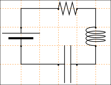
display[{
battery[] // at[{0, 0}, Pi/2],
connect[{{0, 1}, {0, 2}, {2, 2}}],
resistor[] // at[{2, 2}],
connect[{{3, 2}, {4, 2}, {4, 1}}],
coil[] // at[{4, 0}, Pi/2],
connect[{{4, 0}, {4, -1}, {3, -1}}],
capacitor[] // at[{2, -1}],
connect[{{2, -1}, {0, -1}, {0, 0}}]}]
Return to Mathematica page
Return to the main page (APMA0330)
Return to the Part 1 (Plotting)
Return to the Part 2 (First Order ODEs)
Return to the Part 3 (Numerical Methods)
Return to the Part 4 (Second and Higher Order ODEs)
Return to the Part 5 (Series and Recurrences)
Return to the Part 6 (Laplace Transform)
Return to the Part 7 (Boundary Value Problems)
