Return to computing page for the second course APMA0340
Return to computing page for the fourth course APMA0360
Return to Mathematica tutorial for the first course APMA0330
Return to Mathematica tutorial for the second course APMA0340
Return to Mathematica tutorial for the fourth course APMA0360
Return to the main page for the course APMA0330
Return to the main page for the course APMA0340
Return to the main page for the course APMA0360
Return to Part I of the course APMA0330
Glossary
Polar Plots
We use polar coordinates as an alternative way to describe points in the plane. In polar coordinates, we describe points via their angle (called argument or polar angle) with the positive x-axis measured in counterclockwise direction, and the distance from the origin (called radial distance). See figure below.
liner = Graphics[{Red, Thick, Line[{{0, 0}, {1, 1}}]}];
r = Graphics[Text[Style["r", Large, Green], {0.5, 0.6}]];
linex = Graphics[{Orange, Thick, Line[{{0, 0}, {1, 0}}]}];
x = Graphics[Text[Style["x", Large, Black], {0.6, -0.1}]];
y = Graphics[Text[Style["y", Large, Black], {1.1, 0.5}]];
liney = Graphics[{Purple, Thick, Line[{{1, 0}, {1, 1}}]}];
theta = Graphics[Text[Style["\[Theta]", Large, Black], {0.3, 0.1}]];
arc = Graphics[{Blue, Thick, Circle[{0, 0}, 0.2, {0, Pi/4}]}];
arrowx = Graphics[{Arrowheads[0.07], Arrow[{{0, 0}, {1.25, 0}}]}];
arrowy = Graphics[{Arrowheads[0.07], Arrow[{{0, 0}, {0, 1.25}}]}];
Show[{liner, r, linex, x, liney, y, arc, theta, point, arrowx, arrowy}, Ticks -> None, Axes -> True, AxesStyle -> Gray, AxesLabel -> {Style["x", Medium, Gray], Style["y", Medium, Gray]}]
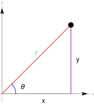
Here are some examples of polar plot.
Cycloid
The Parametrization
Manipulate[
ParametricPlot[
cycloid[a, b][t] // Evaluate, {t, -\[Pi]/2, 5*\[Pi]/2}], {a, 1, 5}, {b, 1, 5}]
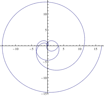
PolarPlot[Cycloid[1.5,theta],{theta, 0, 4*Pi}]
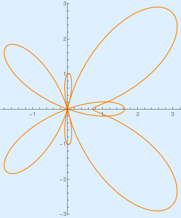
PolarPlot[{Exp[Cos[x]] - 2*Cos[4*x]}, {x, 0, 2*Pi}, PlotStyle -> {Orange}, Background -> LightBlue]
x = r*Cos[\[Theta]]; y = r*Sin[\[Theta]];
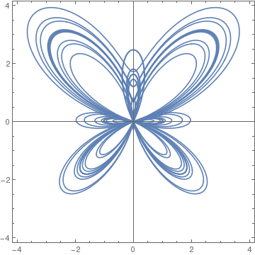
PolarPlot[r, {\[Theta], 0, 24 Pi}, Axes -> True, PlotRange -> {{-4, 4}, {-4, 4}}, Frame -> True, PlotPoints -> 1500, AspectRatio -> Automatic]
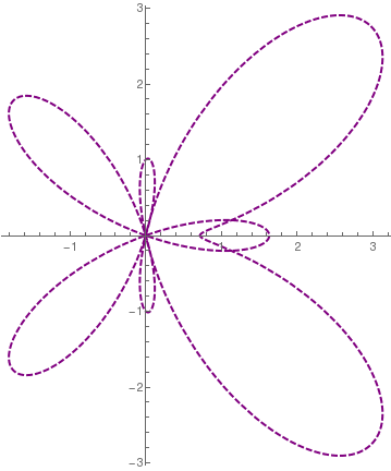
Butterfly curve. |
Butterfly curve with background. |
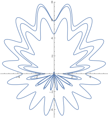
Rotated butterfly curve. |
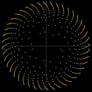
butterfly[99999998][0.0006]
butterfly[\[Lambda]_][h_, o___] := ListPolarPlot[ Table[{\[Theta], (Exp[Cos[\[Theta]]] - 2 Cos[4 \[Theta]])*(Sin[\[Lambda] \[Theta]]^4)}, {\[Theta], 0, 2 Pi, h}], o, PlotRange -> All, PlotStyle -> {PointSize[Tiny], Orange}, Background -> Lighter[LightBlue, 0.25]]
Rotate[%, 90 Degree]
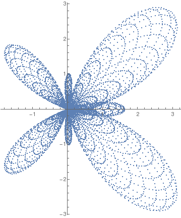
Butterfly curve. |
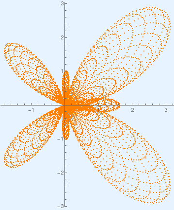
Butterfly curve on background. |
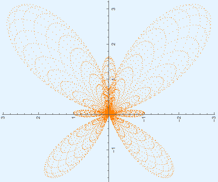
Rotated butterfly curve. |
butterfly[99999998][0.00065]
Rotate[%, 90 Degree]
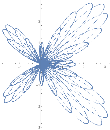
Butterfly curve with step size 0.00065. |
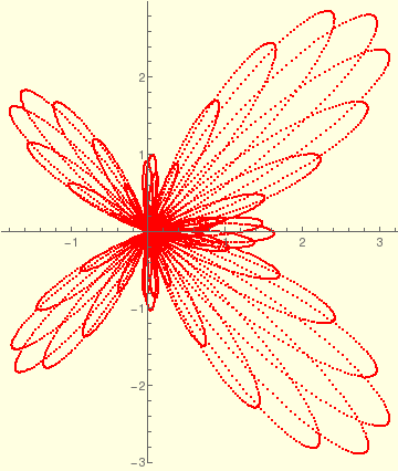
Butterfly curve with step size 0.00065 on background. |
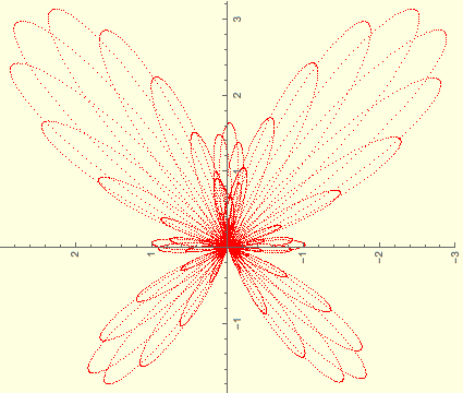
Rotated butterfly curve curve with step size 0.00065. |
butterfly[\[Lambda]_][h_, o___] := ListPolarPlot[ Table[{\[Theta], (Exp[Cos[\[Theta]]] - 2 Cos[4 \[Theta]])*(Sin[\[Lambda] \[Theta]]^4)}, {\[Theta], 0, 2 Pi, h}], o, PlotRange -> All, PlotStyle -> {PointSize[Tiny], Blue}, Background -> LightPink]
butterfly[99999998][0.000169]
Rotate[%, 90 Degree]
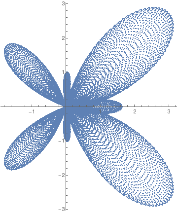
Butterfly curve with step size 0.000169. |

Butterfly curve with step size 0.000169 on background. |
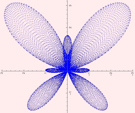
Rotated butterfly curve curve with step size 0.000169. |
Good examples of a polar parametrization are given by some famous spiral curves. In partocular, we mention some of them. The spiral of Archimedes is r = θ.
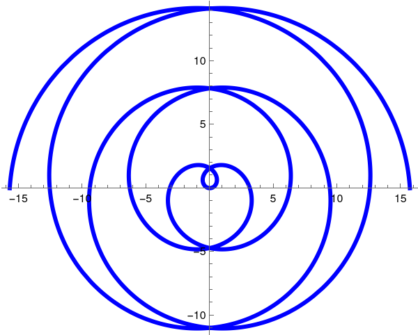
Archimedes apiral. |
Archimedes of Syracuse (287–212 BC) is credited with the
creation of many mechanical devices such as compound pulleys, water
clocks, catapults and burning mirrors. Legend has it that he was killed
by a Roman soldier as he traced mathematical figures in the sand during
the siege of Syracuse, at that time a Greek colony on what is now Sicily.
His mathematical work included finding the area of a circle and the area
under a parabola using the method of exhaustion.
PolarPlot[t, {t, -5*Pi, 5*Pi}, PlotStyle -> Thick]
|
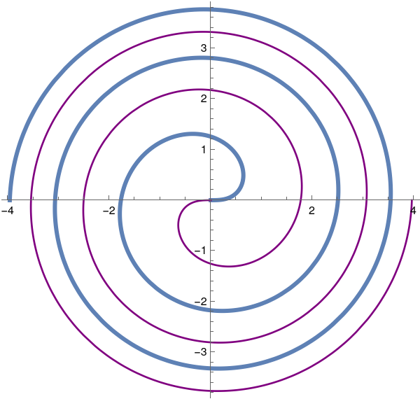
Fermat's apiral. |
Fermat's spiral r = ±√θ has two branches, the second obtained by allowing the
radius function to be negative. The two branches join up provided the exponent
is positive.
Pierre de Fermat (1601–1665), like his contemporary Descartes, was trained as a lawyer. Fermat generalized the work of Archimedes on spirals. Like Archimedes he had the germs of the ideas of both differential and integral calculus – using the new techniques of analytic geometry – but failed to see the connections. Fermat is most remembered for stating the theorem that xn + yn = zn has no solution in integers for n > 2.
PolarPlot[{Sqrt[t], -Sqrt[t]}, {t, 0, 5*Pi},
PlotStyle -> {Thickness[0.01], Purple}]
|
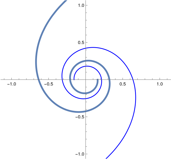
The hyperbolic apiral. |
The hyperbolic spiral r = ±2/θ.
PolarPlot[{2/t, -2/t}, {t, 0.3, 4*Pi},
PlotStyle -> {Thickness[0.01], Blue}]
|
- Abbena, E., Simon, S., Gray, A., Moder Differential Geometry of Curves and Surfaces with Mathematica, Third Edition,
- Geum, Y.H. and Kim, Y.I., On the analysis and construction of the butterfly curve using Mathematica, International Journal of Mathematical Education in Science & Technology, 2008, Vol. 39, Issue 5, pp. 670--678.
- Fay. T., The Butterfly curve, The American mathematical Monthly, 1989, Vol. 96, No 5, pp. 142--143.
- Fay. T., A study in step size, Mathematics magazine, 1997, Vol. 70, No. 2, pp. 116--117.
Return to Mathematica page
Return to the main page (APMA0330)
Return to the Part 1 (Plotting)
Return to the Part 2 (First Order ODEs)
Return to the Part 3 (Numerical Methods)
Return to the Part 4 (Second and Higher Order ODEs)
Return to the Part 5 (Series and Recurrences)
Return to the Part 6 (Laplace Transform)
Return to the Part 7 (Boundary Value Problems)