Return to computing page for the second course APMA0340
Return to Mathematica tutorial for the second course APMA0340
Return to the main page for the course APMA0330
Return to the main page for the course APMA0340
Return to Part I of the course APMA0330
Glossary
Labeling Figures
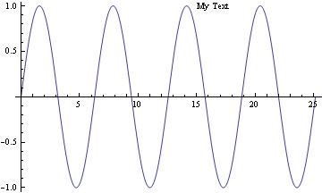
Label lines: To see the equation of the line when cursor reaches the graph, use Tooltip command:
|
Plot[Tooltip[Sin[x]], {x, 0, 8 Pi}]
To put text/title on the picture, use Epilog command: Plot[Sin[x], {x, 0, 8 Pi}, Epilog -> Text["My Text", Offset[{32, 0}, {14, Sin[14]}]]] |
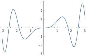
You can put title below the graph.
|
Clear[x];
Labeled[Plot[Sin[x^2] x, {x, -3, 3}, ImageSize -> 300], Text@TraditionalForm@Style[Sin[x*x], 16]] |
|
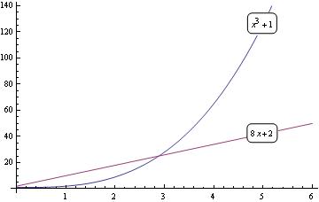
To write labels on the graph:
fns[x_] := {1 + x^3, 2 + 8*x};
len := Length[fns[x]]; Plot[Evaluate[fns[x]], {x, 0, 6}, Epilog -> |
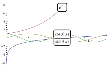
You can do something similar with Locators that allows you to move the labels wherever you want:
|
fns[x_] := {Log[x], Exp[2*x], Sin[4*x], Cos[6*x]}; DynamicModule[{pos = Table[{1, fns[1][[i]]}, {i, len}]}, |
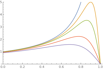
You can use PlotLagends (that are not visible on the graph, but in Mathematica notebok):
|
f[a_, x_] := 1/((1 - x) (1 + a/(1 - x)^2));
parameters = {0, 0.01, 0.02, 0.05, 0.1}; Plot[Evaluate[f[#, x] & /@ parameters], {x, 0, 1}, PlotRange -> {0, 5}, PlotLegends -> Table[Row[{"a=", j}], {j, parameters}]] |
Instead of
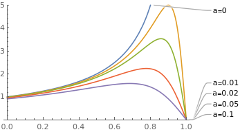
PlotLagends, you can use PlotLabels
|
f[a_, x_] := 1/((1 - x) (1 + a/(1 - x)^2));
parameters = {0, 0.01, 0.02, 0.05, 0.1}; Plot[Evaluate[f[#, x] & /@ parameters], {x, 0, 1}, PlotRange -> {0, 5}, PlotLabels -> Table[Row[{"a=", j}], {j, parameters}]] |
Plotting with axes and without axes
There are times when the axes could interfere with displaying certain functions and solutions to ODEs. Fortunately, getting rid of axes in recent versions of Mathematica is very easy.
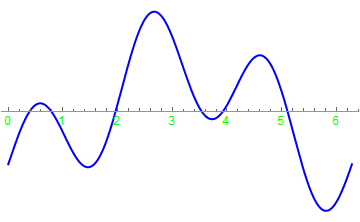
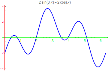
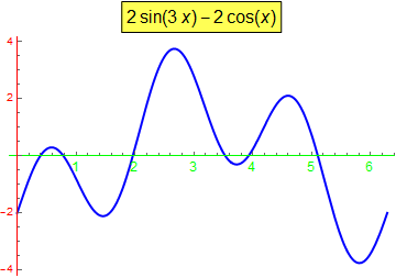
One method of specifying axes is to use the above options, but there is also a visual method of changing axes. Let us plot the function \( f(x) = 2\,\sin 3x -2\,\cos x \) without ordinate but using green color and font size 12 for abscissa:
|
f[x_] = 2*Sin[3*x] - 2*Cos[x]
Plot[f[x], {x, 0, 2*Pi}, PlotStyle -> {Thick, Blue}, Axes -> {True, False}, AxesStyle -> Directive[Green, 12]] |
One can also use different colors and fonts for different axes.
 |
Plot[f[x], {x, 0, 2*Pi}, PlotStyle -> {Thick, Blue}, Axes -> {True},
AxesStyle -> {Directive[Green, 12], Red}]
|
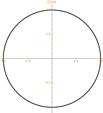
We can plot two graphs in the same figure:
 |
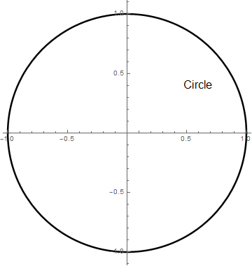 |
AxesStyle -> {Directive[Green, 12], Red}, PlotLabel -> 2*Sin[3*x] - 2*Cos[x]] Plot[f[x], {x, 0, 2*Pi}, PlotStyle -> {Thick, Blue}, Axes -> {True},
AxesStyle -> {Directive[Green, 12], Red},
PlotLabel -> Style[Framed[2*Sin[3*x] - 2*Cos[x]], 16, Black, Background -> Lighter[Yellow]]]
 |
 |
We show how to present data using GraphicsGrid command:

Return to Mathematica page
Return to the main page (APMA0330)
Return to the Part 1 (Plotting)
Return to the Part 2 (First Order ODEs)
Return to the Part 3 (Numerical Methods)
Return to the Part 4 (Second and Higher Order ODEs)
Return to the Part 5 (Series and Recurrences)
Return to the Part 6 (Laplace Transform)
Return to the Part 7 (Boundary Value Problems)