The modified decomposition method (MDM) is
both a decelerated Adomian decomposition method and a developed power series method that nicely and accurately treats any analytic nonlinearity in differential equations. In case of autonomous homogeneous or nonhomogeneous equations, the method is seemed to be superior over other methods. Therefore, we start demonstration of this method in initial value problems for first order differential equations of the form
\begin{equation} \label{Eqmdm1.1}
L \left[ y(t) \right] = N\left[ y(t) \right] + g(t) ,
\qquad y(t_0 ) = y_0 ,
\end{equation}
where
\( L \left[ y(t) \right] = y' (t) + a (t)\, y (t) = {\text d}y/{\text d}t + a (t)\, y (t) \) is the linear differential operator,
\( N \left[ y(t) \right] \) is a nonlinear term, and
g is the system input and
y is the system output. The differential operator can be rewritten as
\( L = \texttt{D} + a(t)\,\texttt{I} \) , where
\( \texttt{D} = {\text d}/{\text d}t \) is the derivative operator and
\( \texttt{I} \) is the identical operator. Since the unbounded derivative operator has a one-dimensional kernel (the set of functions that are annihilated by the derivative operator), its inverse, calling antiderivative, is a multi-valued operator depending on some constant. Similar property is valid for
L . In order to knock out a single inverse operator
L -1 , we consider
L on a space of functions that satisfy an initial condition; more over, it is assumed that an explicit formula for it is available.
Furthermore, we emphasize that the choice for
L and concomitantly its
inverse
L -1 are determined by the particular equation to be
solved. Hence, the choice for
L is nonunique, e.g., for cases of differential
equations with singular coefficients, a different form for the linear
operator
L can be chosen. As a rule, the highest derivative is taken
as the linear operator
L . Later we consider more general equation including coefficients depending on independent variable.
The Rach--Adomian--Meyers MDM decomposes the solution into a power series
\begin{equation} \label{Eqmdm1.2}
y(t) = \sum_{n\ge 0} c_n \left( t- t_0 \right)^n
\end{equation}
and decomposes the nonlinearity into a power series
according to the Adomian--Rach theorem
\[
N \left[ y(t) \right] = N \left[ \sum_{n\ge 0} c_n \left( t- t_0 \right)^n \right] = \sum_{n\ge 0} A_n \left( c_0 , c_1 , \ldots , c_n \right) \left( t- t_0 \right)^n ,
\]
where
A n are the Adomian polynomials in terms of solution coefficients. Of course, the above formula is nothing more than Taylor's series expansion of the nonlinear function
N [
y ]. However, the main difference of the MDM expansion from the power series is that in the former the coefficients depend recursively on the previous coefficients whereas Taylor's coefficients all depend on the infinitesimal behavior of the slope function, but not on previously found coefficients. It is convenient to make a shift in independent variable
x =
t -
t 0 to transfer the initial point from
t 0 into the origin:
\[
y(x) = y_0 + \sum_{n\ge 1} c_n \, x^n \qquad\mbox{and} \qquad N \left[ y(x) \right] = \sum_{n\ge 0} A_n \left( c_0 , c_1 , \ldots , c_n \right) x^n .
\]
The Adomian polynomials are evaluated in a similar way as in the ADM
\[
A_n = \frac{1}{n!} \, \frac{\partial^n}{\partial \lambda^n} \left( N\left[
\sum_{n\ge 0} u_n \lambda^n \right] \right)_{\lambda =0} , \qquad n=0,1,2,\ldots ;
\]
but with substitution
c n instead of
u n :
\[
A_n \left( u_0 , u_1 , \ldots , u_n \right) = x^n A_n \left( c_0 , c_1 , \ldots , c_n \right) , \qquad n=0,1,2,\ldots .
\]
Mathematica code for evaluating Adomian polynomials (Jun-Sheng Duan, An efficient algorithm for the multivariable Adomian polynomials,
Applied Mathematics and Computation , 2010, 217, pp. 2456--2467):
Adom1[n_]:= Module[{A, Z, dir},
Here is its another version (Jun-Sheng Duan):
Adom2[n_] := Module[{pol, A},
We begin with the
Adomian form of the ordinary differential equation, but instead employ the Taylor expansion series for the solution and the
nonlinear function of the solution. The later is possible because of the nonlinear transformation of series by the Adomian–
Rach Theorem
Michaelis--Menten (MM) equation
Example: Michaelis--Menten equation (MM for short) is employed to describe the kinetics of enzyme-catalysed reactions. Enzymesare proteins that catalyse the chemical reactions essential for living organisms. Therefore, we will solve the MM equation
\[
s' (r) = - \frac{V_m s(r)}{K_m + s(r)} , \qquad s(0) = a,
\]
where
s (
r ) is the substrate concentration,
V m and
K m are the limiting rate and Michaelis constant, respectively. In general,the explicit closed form of the solution is
\[
s(r) = K_m W \left\{ \frac{a}{K_m} \,\exp \left( \frac{a - V_m r}{K_m} \right) \right\} ,
\]
where
W is the
Lambert function and 𝑎 is a constant value from initial condition that satisfies according to the IVP.
We apply the modified decomposition method assuming that the solution is represented by a convergent power series
\[
s(r) = \sum_{n\ge 0} c_n r^n = a + \sum_{n\ge 1} c_n r^n ,
\]
where the initial term matches the initial condition. The nonlinearity is expanded into the Adomian series
\[
f(s) = - \frac{V_m s}{K_m + s} = \sum_{n\ge 0} A_n r^n ,
\]
where
\begin{align*}
A_0 &= f(a) = - \frac{V_m a}{K_m + a} ,
\\
A_1 &= c_1 f' (a) = -\frac{K_m V_m c_1}{\left( K_m +a \right)^2} ,
\\
A_2 &= \frac{K_m V_m c_1^2 - K_m^2 V_m c_2 - K_m V_m a\,c_2}{\left( K_m +a \right)^3} ,
\\
A_3 &= \frac{K_m V_m c_1 c_2 - V_m c_1^3 + V_m a\,c_1 c_2}{\left( K_m +a \right)^3} + \frac {V_m a \,c_1^3 - 2V_m a\, c_1 c_2}{\left( K_m + a \right)\left( K_m +a \right)^3} + \frac{V_m c_1 c_2}{\left( K_m +a \right)^2} + \frac{V_m a\,c_3}{\left( K_m +a \right)^2} - \frac{V_m c_3}{\left( K_m +a \right)} ,
\\
A_4 &=
\\
A_5 &=
\end{align*}
Substituting these series into the MM equation, we obtain
\[
\sum_{n\ge 1} n\,c_n r^{n-1} = \sum_{n\ge 0} n\,A_n r^{n} .
\]
This allows us to derive the recurrence relation to determine the values of unknown coefficients:
\begin{align*}
c_1 &= A_0 = - \frac{V_m a}{K_m + a} ,
\\
2\, c_2 &= A_1 = \frac{K_m V_m^2 a\, c_1}{\left( K_m +a \right)^3} ,
\\
3\, c_3 &= A_2
\\
4\,c_4 &= A_3
\end{align*}
Now we make a numerical experiment by choosing particular values of coefficients:
\[
K_m =1 , \qquad a = 2, \qquad V_m =3.
\]
Then the Adomian polynomial becomes
f[y_] = -3*y/(1 + y);
\[
f(s) = - \frac{V_m s}{K_m + s} = -2 - \frac{c_1}{3}\, r + \left( \frac{c_1^2}{9} - \frac{c_2}{3} \right) r^2 + \left( \frac{2\,c_1 c_2}{9} - \frac{c_1^3}{27} - \frac{c_3}{3} \right) r^3 + \left( \frac{c_1^4}{81} + \frac{c_2^2 - c_1^2 c_2 + 2\,c_1 c_3}{9} - \frac{c_4}{3} \right) r^4 + \left( -\frac{c_1^5}{243} + \frac{4}{81}\,c_1^3 c_2 + \frac{2\,c_1 c_4 + 2\,c_2 c_3 - c_1^2 c_3 -c_1 c_2^2}{9} - \frac{c_5}{3} \right) r^5 + \cdots .
\]
From the above recurrence relations, we find numerical values of the MDM coefficients:
\begin{align*}
c_1 &= -2,
\\
c_2 &= \frac{1}{3} ,
\\
c_3 &= \frac{1}{9} ,
\\
c_4 &= \frac{1}{36} ,
\\
c_5 &= \frac{1}{1620} ,
\\
c_6 &= - \frac{47}{9720} .
\end{align*}
We compare these coefficients with the Taylor series expansion
AsymptoticDSolveValue[{s'[r] == -3*s[r]/(1 + s[r]), s[0] == 2},
s[r], {r, 0, 9}]
2 - 2 r + r^2/3 + r^3/9 + r^4/36 + r^5/1620 - (47 r^6)/9720 - (
247 r^7)/68040 - (2581 r^8)/1632960 - (4429 r^9)/14696640
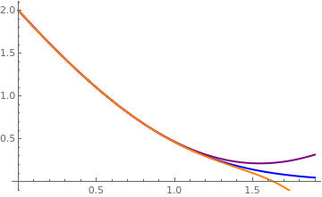
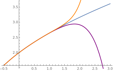
Explicit solution (in blue) and two polynomial approximations.
Sol = NDSolve[{y'[x] == -3*y[x]/(1+y[x]) , y[0] == 2}, y, {x, 0, 1.9}];
■
We rewrite the first order equation \eqref{Eqmdm1.1} in explicit way.
Once we expand into Maclauirin power series every term in the given differential equation (assuming that shifting of independent variable was done)
\begin{equation} \label{Eqmdm1.3}
\frac{{\text d}y}{{\text d}x} + a(x)\,y(x) = N \left[ y(x) \right] + g(x)
\end{equation}
we obtain
\[
\sum_{k\ge 1} c_k \,k \,x^{k-1} + \left( \sum_{k\ge 0} a_k x^k \right) \left( \sum_{k\ge 0} c_k x^k \right) = \left( \sum_{k\ge 0} b_k x^k \right) \left( \sum_{k\ge 0} c_k x^k \right) + \sum_{k\ge 0} A_k \left( c_0 , \ldots , c_k \right) x^k + \sum_{k\ge 0} g_k x^k ,
\]
where coefficients
c k are unknown yet. Using the convolution rule for power series (also known as
Cauchy product ), we get
\[
\sum_{k\ge 1} c_k \,k \,x^{k-1} + \sum_{k\ge 0} \left( \sum_{i=0}^k a_{k-i} c_i \right) x^k = \sum_{k\ge 0} \left( \sum_{i=0}^k b_{k-i} c_i \right) x^k + \sum_{k\ge 0} A_k \left( c_0 , \ldots , c_k \right) x^k + \sum_{k\ge 0} g_k x^k .
\]
Then equating coefficients of like powers of
x , we derive a recurrence relation for determination of unknown coefficients
c k .
\[
c_{k+1} \left( k+1 \right) + \sum_{i=0}^k a_{k-i} c_i = \sum_{i=0}^k b_{k-i} c_i + A_k \left( c_0 , \ldots , c_k \right) + g_k , \quad c_0 = y(0) , \qquad k=0,1,2,\ldots .
\]
Since we are working with holomorphic functions , it is natural to assume that the input function g is represented by a convergent power series
\[
g(x) = \sum_{n\ge 0} g_n \frac{x^n}{n!} .
\]
Substituting all these series into the differential equation, we obtain
\begin{align*}
L \left[ y(x) \right] &= \texttt{D} \sum_{n\ge 1} c_n x^n + a(x)\,\sum_{n\ge 0} c_n x^n = \sum_{n\ge 1} n\,c_n x^{n-1} + \left( \sum_{n\ge 0} \alpha_n x^n \right) \left( \sum_{n\ge 0} c_n x^n \right) ,
\\
R \left[ y(x) \right] &= b(x)\,y(x) = \left( \sum_{n\ge 0} \beta_n x^n \right) \left( \sum_{n\ge 0} c_n x^n \right) ,
\\
N \left[ y(x) \right] &= \sum_{n\ge 0} A_n x^n .
\end{align*}
Since the multiplication of two series leads to their convolution,
\[
\left( \sum_{n\ge 0} a_n x^n \right) \left( \sum_{n\ge 0} b_n x^n \right) =
\sum_{n\ge 0} \left( \sum_{k=0}^n a_k b_{n-k} \right) x^n
\]
we get the equation for power series:
\[
\sum_{n\ge 1} n\,c_n x^{n-1} + \sum_{n\ge 0} \left( \sum_{k=0}^n \alpha_k c_{n-k} \right) x^n = \sum_{n\ge 0} \left( \sum_{k=0}^n \beta_k c_{n-k} \right) x^n + \sum_{n\ge 0} A_n x^n + \sum_{n\ge 0} g_n \frac{x^n}{n!} ,
\]
with
\[
c_0 = y_0 .
\]
Example: first order self-adjoint differential operator
Example:
\[
\frac{{\text d}y}{{\text d}x} + 2x\, y(x) = 2 + 2\,x^2 + \frac{y^2}{2} , \qquad y(0) =1.
\]
The given problem has the explicit solution
\[
y(x) = 2x + \frac{1}{1-x/2} = 1 + \frac{5x}{2} + \frac{x^2}{4} + \frac{x^3}{8} + \left( \frac{x}{2} \right)^4 + \left( \frac{x}{2} \right)^5 + \left( \frac{x}{2} \right)^6 + \cdots + \left( \frac{x}{2} \right)^n + \cdots .
\]
which we verify with
Mathematica :
y[x_] = 2*x + 1/(1 - x/2);
0
Series[y[x], {x, 0, 10}]
Let
L be the differential operator
\[
L\left[ x, \texttt{D} \right] = e^{-x^2} \texttt{D} e^{x^2} = \texttt{D} + 2x\,\texttt{I} \qquad \Longrightarrow \qquad L^{-1}\left[ x, \texttt{D} \right] f(x) = y(0)\,e^{-x^2} + e^{-x^2} \int_0^x e^{s^2} f(s)\,{\text d}s ,
\]
and
\( N\left[ y \right] = y^2 \) be the nonlinear operator. Then we rewrite the given problem in the operator form:
\[
L\left[ x, \texttt{D} \right] y = 2 + 2\,x^2 + \frac{1}{2}\,N\left[ y \right]
\]
Assuming that the solution can be decomposed into convergent power series
\[
y(x) = 1 + \sum_{n\ge 1} c_n x^n ,
\]
we expand the nonlinear term into the series :
\[
N \left[ y \right] = y^2 = N \left[ 1 + \sum_{n\ge 1} c_n x^n \right] = \sum_{n\ge 0} A_n \left( 1, c_1 , \ldots , c_n \right) x^n ,
\]
where
\( A_n = \sum_{k=0}^n c_k c_{n-k} \) are the Adomian's polynomials. Substituting these series into the given differential equation, we get
\begin{align*}
L\left[ x, \texttt{D} \right] y(x) &= \sum_{n\ge 1} n\,c_n x^{n-1} + 2x + 2
\sum_{n\ge 1} c_n x^{n+1} = 2 + 2\,x^2 + \frac{1}{2} \sum_{n\ge 0} A_n x^n .
\end{align*}
The first Adomian polynomails should be
\[
A_0 = 1 = N\left[ 1 \right]
\]
because of the initial condition
y (0) = 1 =
c 0 . Now we compare coefficients of like powers and obtain the sequence of recurrence relations:
\begin{align*}
c_1 &= 2 + \frac{1}{2}\, A_0 = \frac{5}{2} , \\
2\,c_2 +2 &= \frac{1}{2}\, A_1 = c_1 c_0 \qquad \Longrightarrow \qquad c_2 = \frac{1}{4} , \\
3\, c_3 + 2\, c_1 &= 2 + \frac{1}{2}\, A_2 = 2 + c_0 c_2 + \frac{1}{2}\, c_2^2 \qquad \Longrightarrow \qquad c_3 = \frac{1}{8} ,
\\
\left( n+1 \right) c_{n+1} + 2\,c_{n-1} &= \frac{1}{2}\, A_n , \qquad n= 3,4, \ldots .
\end{align*}
Therefore, we get a recurrence:
\[
c_{n+1} = \frac{1}{2(n+1)} \, A_n \left( 1, c_1, c_2 , \ldots , c_n \right) - \frac{2}{n+1}\, c_{n-1} = \frac{1}{2^{n+1}} , \qquad n=3,4,\ldots .
\]
This formulas can be verified by induction.
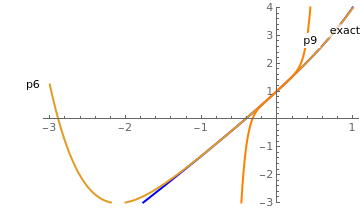
Explicit solution and two polynomial approximations.
ss[x_] = 2*x + 1/(1 - x/2);
p6[t_] = 1 + 5*t/2 + t^2 /4 + t^3/8 + t^4/2^4 + t^5/2^5 + t^6/2^6;
■
Example: nonlinear equation
Example: holomorphic function
\[
\frac{{\text d} y}{{\text d}x} +2x\,f \left( y(x) \right) = 3x, \qquad y(0) =1,
\]
where
f is a known function having required number of derivatives (generally speaking, all derivatives). Assuming that the given differential equation has a convergent Maclaurin series solution
\[
y(x) = \sum_{n\ge 0} c_n x^n = 1 + \sum_{n\ge 1} c_n x^n ,
\]
we expand the nonlinear term into Adomian's series
\[
f \left( y(x) \right) = \sum_{n\ge 0} A_n \left( c_0 , c_1 , \ldots , c_n \right) x^n = \sum_{n\ge 0} A_n x^n .
\]
Taking the derivative, we get
\[
y' (x) = \sum_{n\ge 0} (n+1)\, c_{n+1} x^n .
\]
Similar, we expand the nonlinear term:
\[
x\,f \left( y(x) \right) = \sum_{n\ge 0} A_n \left( c_0 , c_1 , \ldots , c_n \right) x^{n+1} = A_0 x + \sum_{n\ge 0} A_{n+1} x^{n+2} ,
\]
where
A n are Adomian's polynomials for the nonlinearity
N [
y ].
Substituting these identities into the given differential equation, we obtain
\[
c_1 + 2\,c_2 x + \sum_{n\ge 0} \left( n+3 \right) c_{n+3} x^{n+2} = 3x - 2\,A_0 x -2\,\sum_{n\ge 0} A_{n+1} x^{n+2} .
\]
From the initial condition, we find immediately that
c 0 = 1, and for all other coefficients, we get the recurrence relation by equating the coefficients of like powers of
x :
\begin{align*}
c_1 &= 0 ,
\\
2\,c_2 &= 3 - 2\, A_0 = 3 - 2\, f(c_0 ) \qquad \Longrightarrow \qquad c_2 = \frac{1}{2} \left( 3 - 2\,N(1) \right) ,
\\
c_{n+3} &= - \frac{2}{n+3} \, A_{n+1} , \qquad n= 2,3,\ldots .
\end{align*}
The truncated sum
\[
\phi_m (x) = \sum_{k=0}^m c_k x^k = 1 + \sum_{k=1}^m c_k x^k
\]
gives a polynomial approximation to the solution.
■
Example: Riccati equation
Example:
\[
\frac{{\text d} y}{{\text d}x} = x^2 + y^2 (x), \qquad
y(x_0 ) = y_0 =1.
\]
Its solution is expressed through
Bessel functions :
\[
y(x) = \begin{cases}
-x\,\frac{J_{-3/4} \left( \frac{x^2}{2} \right) \left( \Gamma^2 \left( \frac{3}{4} \right) + \pi \right) - Y_{-3/4} \left( \frac{x^2}{2} \right)\Gamma^2 \left( \frac{3}{4} \right) }{\left( \Gamma^2 \left( \frac{3}{4} \right) + \pi \right) J_{1/4} \left( \frac{x^2}{2} \right) - Y_{1/4} \left( \frac{x^2}{2} \right)\Gamma^2 \left( \frac{3}{4} \right) } , & \ x< 0,
\\
1, & \ x = 0,
\\
-x\,\frac{J_{-3/4} \left( \frac{x^2}{2} \right) \left( -\Gamma^2 \left( \frac{3}{4} \right) + \pi \right) + Y_{-3/4} \left( \frac{x^2}{2} \right)\Gamma^2 \left( \frac{3}{4} \right) }{\left( -\Gamma^2 \left( \frac{3}{4} \right) + \pi \right) J_{1/4} \left( \frac{x^2}{2} \right) + Y_{1/4} \left( \frac{x^2}{2} \right)\Gamma^2 \left( \frac{3}{4} \right) } , & \ x> 0.
\end{cases}
\]
Its series solution can also be found with
Mathematica :
AsymptoticDSolveValue[{y'[x] == y[x]*y[x] + x^2, y[0] == 1},
y[x], {x, 0, 9}]
\[
y(x) = 1 + x + x^2 + \frac{3}{4}\,x^3 + \frac{7}{6}\,x^4 + \frac{6}{5}\,x^5 + \frac{37}{30}\,x^6 + \frac{404}{315}\,x^7 + \frac{369}{280}\,x^8 + \frac{428}{315}\,x^9 + O\left( x^{10} \right) .
\]
It is convenient to rewrite the given differential equation in operator form:
\[
L\left[ y \right] = f(y) + g(x) ,
\]
where
\[
L\left[ y \right] = \texttt{D}\,y(x) = \frac{{\text d} y}{{\text d}x} ,
\qquad g(x) = x^2 , \quad f(y) = y^2 (x) .
\]
The inverse of the unbounded differential operator
L = D dependends on an arbitrary constant, which we denote as
c :
\[
L^{-1} \left[ u \right] = c + \int_{x_0}^x
u(t)\,{\text d}t .
\]
Application of the bounded operator to the given differential equation yields
the functional equation for which the fixed point theorem can be applied:
\[
y(x) = L^{-1} \left[ g(x) \right] + L^{-1} \left[ f(y) \right] .
\]
The Adomian decomposition method (ADM) states
that the dependent variable
y (
x ) and the nonlinear term
f (
y ) =
y ² should be written as the following
infinite series
\begin{align*}
y(x) &= \sum_{n\ge 0} u_n (x) ,
\\
f(y(x)) &= \sum_{n\ge 0} A_n \left( u_0 , u_1 , u_2 , \ldots , u_n \right) ,
\end{align*}
where
A k is the
k -th Adomian polynomial. Instead of the standard ADM, we apply the modified decomposition method, which is based on power series expansion
\begin{align*}
y(x) &= \sum_{n\ge 0} c_n \,x^n = 1 + \sum_{n\ge 1} c_n \,x^n ,
\\
f(y(x)) &= \sum_{n\ge 0} A_n \left( c_0, c_1 , c_2 , \ldots , c_k \right) x^k .
\end{align*}
For a quadratic function
f =
x ², the Adomian polynomials were calculated previously in
section :
\begin{align*}
A_0 &= f(1) = 1,
\\
A_1 &= 2\,c_1 ,
\\
A_2 &= c_1^2 + 2\,c_2 ,
\\
A_3 &= 2\,c_1 c_2 + 2\,c_3 ,
\\
A_4 &= c_2^2 + 2\, c_1 c_3 + 2\,c_4 ,
\\
A_5 &= 2\,c_2 c_3 + 2\,c_1 c_4 + 2\,c_5 ,
\\
A_6 &= c_3^2 + 2\,c_2 c_4 + 2\,c_1 c_5 + 2\,c_6 .
\end{align*}
Substituting the power series into the given Riccati equation, we obtain
\[
\sum_{n\ge 1} n\,c_n x^{n-1} = \sum_{n\ge 0} A_n x^n + x^2
\]
This leads ato a sequence of recurrence relations:
\begin{align*}
c_1 &= A_0 = 1,
\\
2\,c_2 &= A_1 = 2 \qquad \Longrightarrow c_2 = 1,
\\
3\,c_3 &= A_2 + 1 = 4 \qquad \Longrightarrow c_3 = \frac{4}{3} ,
\\
4\,c_4 &= A_3 = \frac{14}{3} \qquad \Longrightarrow c_4 = \frac{7}{6} ,
\\
5\,c_5 &= A_4 = 6 \qquad \Longrightarrow c_5 = \frac{6}{5} ,
\\
6\,c_6 &= A_5 = \frac{37}{5} \qquad \Longrightarrow c_6 = \frac{37}{30} .
\end{align*}
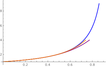
Explicit solution and two polynomial approximations.
ss[x_] = -x*(BesselJ[-3/4, x^2/2] *(-Gamma[3/4]^2 + Pi) +
BesselY[-3/4, x^2/2] *Gamma[3/4]^2)/((-Gamma[3/4]^2 + Pi)*
BesselJ[1/4, x^2/2] + BesselY [1/4, x^2/2] *Gamma[3/4]^2);
{x -> 0.969811}
■
Example: Exponential slope function
Example:
\[
y' = e^y -2\, \tan (2x) - \cos (2x), \qquad y(0) =0;
\]
that has the true solution
\( y(x) = \ln \left( \cos 2x \right) . \) Mathematica confirms
u[x_] = Log[Cos[2*x]]
D[u[x], x] + 2*Tan[2*x] + Cos[2*x] - Exp[u[x]]
With
Mathematica , we find its power series expansion to be
Series[Log[Cos[2*x]], {x, 0, 12}]
\[
y(x) = -2x^2 - \frac{4}{3}\, x^4 - \frac{64}{45}\, x^6 - \frac{544}{315}\, x^8 - \frac{1415168}{46777}\, x^{10} - \frac{1415168}{467775}\, x^{12} - \cdots .
\]
According to the standard ADM, we assume that solution is represented by infinite series
\[
y(x) = u_0 (x) + \sum_{k\ge 1} u_k (x) ,
\]
where The components
u n (
x ) are solutions of the initial value problems
\[
u'_n =A_{n-1}\left( u_0 , u_1 , \ldots u_{n-1} \right) , \qquad u_n (0) = 0 , \quad n=1,2,\ldots ,
\]
and the initial term is determined from the IVP:
\[
u'_0 = \tan (2x) - \cos (2x), \qquad y(0) =0.
\]
Integrate[Tan[2*s] - Cos[2*s], s]
So
\[
u_0 (x) = - \frac{1}{2}\,\ln \left[ \cos (2x) \right] - \frac{1}{2}\,\sin (2x) .
\]
All other components are determined recursively by solving the initial value problems subject that the Adomian polynomials are available. Using the nonlinear term
N [
y ] = e
y , we get the first Adomian polynomial directly
\[
A_0 (u_0 ) = N[ u_0 ] = e^{u_0} = e{- \frac{1}{2}\,\ln \left[ \cos (2x) \right] - \frac{1}{2}\,\sin (2x)} = \frac{1}{\sqrt{\cos 2x}}\,e^{- \sin (2x)/2} .
\]
However, we are not going to apply the Adomian decomposition method, but its modification. So we are lokking for its solution in terms of power series
\[
y(x) = c_0 + c_1 x + c_2 x^2 + \cdots = \sum_{n\ge 1} c_n x^n , \qquad\mbox{and} \qquad y' (x) = \sum_{n\ge 1} n\,c_n x^{n-1} ,
\]
where the initial term
u 0 = 0 is set to zero due to the initial condition
y (0) = 0. Next, we expand the input term and the nonlinearity into the power series:
\begin{align*}
-2\,\tan (2x) - \cos (2x) &= -1 - 4x + 2x^2 - \frac{16}{3}\, x^3 - \frac{2}{3}\, x^4 - \frac{128}{15}\, x^5 + \frac{4}{45}\, x^6 - \frac{4352}{315}\, x^7 + \cdots ,
\\
e^y &= A_0 (c_0 ) + A_1 \left( c_0 , c_1 \right) x + A_2 \left( c_0 , c_1 , c_2 \right) x^2 + \cdots .
\end{align*}
Series[Tan[2*x] - Cos[2*x], {x,0,7}]
Since
\( A_0 (c_0 ) = e^{c_0} = e^0 = 1 , \) we get the first component
\[
c_1 = e^{c_0} -1 =1-1 = 0 .
\]
The Adomian coefficients for the nonlinearity are
\begin{align*}
A_1 &= c_1 e^{c_0} = 0 ,
\\
A_2 &= \left( \frac{1}{2}\, c_1^2 + c_2 \right) e^{c_0} = c_2 ,
\\
A_3 &= \left( \frac{1}{6}\, c_1^3 + c_1 c_2 + c_3 \right) e^{c_0} = c_3 ,
\\
A_4 &= \left( \frac{1}{24}\, c_1^4 + \frac{1}{2} \,c_1^2 c_2 + \frac{1}{2}\, c_2^2 + c_1 c_3 + c_4 \right) e^{c_0} = \frac{1}{2}\, c_2^2 + c_4 ,
\\
A_5 &= \left( \frac{1}{120}\, c_1^5 + \frac{1}{6} \,c_1^3 c_2 + \frac{1}{2} \,c_1 c_2^2 + \frac{1}{2}\, c_1^2 c_3 + c_2 c_3 + c_1 c_4 + c_5 \right) e^{c_0} = c_2 c_3 + c_5 ,
\end{align*}
and so on. Substituting these series into the given differential equation, we obtain
\[
2\,c_2 x + 3\,c_3 x^2 + 4\,c_4 x^3 + 5\,c_5 x^4 + 6\,c_6 x^5 + \cdots = c_2 x^2 + c_3 x^3 + \left( \frac{1}{2}\, c_2^2 + c_4 \right) x^4 + \left( c_2 c_3 + c_5 \right) x^5 + \cdots - 4x + 2x^2 - \frac{16}{3}\, x^3 - \frac{2}{3}\, x^4 - \frac{126}{15}\, x^5 + \cdots .
\]
Equating coefficients of like power of
x , we derive the system of recursive relations:
\begin{align*}
2\,c_2 &= -4, \qquad \Longrightarrow \qquad c_2 = -2,
\\
3\,c_3 &= c_2 + 2 = 0, \qquad \Longrightarrow \qquad c_3 = 0,
\\
4\,c_4 &= c_3 - \frac{16}{3}, \qquad \Longrightarrow \qquad c_4 = - \frac{4}{3} ,
\\
5\,c_5 &= \frac{1}{2}\, c_2^2 + c_4 - \frac{2}{3} , \qquad \Longrightarrow \qquad c_5 = 0,
\\
6\,c_5 &= c_2 c_3 + c_5 - \frac{126}{15} ,\qquad \Longrightarrow \qquad c_6 = \frac{4}{45} ,
\end{align*}
and so on. Hence, we get a 5-th degree polynomial approximation.
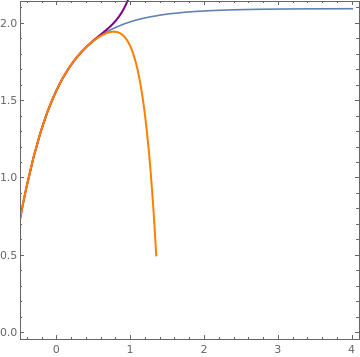
Explicit solution and two polynomial approximations.
s = ContourPlot[
1/Sqrt[3]*Tan[z/2] ==
Tanh[0.658478948462408 + x*Sqrt[3]/2], {x, -0.4, 4}, {z, 0, 2.1}]
■
General first order differential equation
We consider the following initial value problem for the nonlinear differential equation with
holomorphic input function
g (
x ) and holomorphic coefficients
\[
\frac{{\text d}y}{{\text d}x} = a(x)\,y(x) + b(x)\,N \left[ y(x) \right] + g(x) , \qquad y(0) = y_0 .
\]
We assume that this problem has a Maclaurin power series solution
\[
y (x) = c_0 + \sum_{k\ge 1} c_k \,x^k , \qquad \mbox{with} \quad c_0 = y(0) = y_0 .
\]
Since all known functions in the above differential equation are holomorphic, we have
\begin{align*}
a(x) &= \sum_{k\ge 0} a_k x^k ,
\\
b(x) &= \sum_{k\ge 0} b_k x^k ,
\\
g(x) &= \sum_{k\ge 0} g_k x^k ,
\\
,N \left[ y(x) \right] &= \sum_{n\ge 0} A_n \left( c_0, c_1 , \ldots , c_n \right) x^n ,
\end{align*}
where
A n are the Adomian polynomials corresponding to the nonlinearity. Substituting these series into the given differential equation, we obtain the equation between series:
\[
\sum_{k\ge 1} k\,c_k x^{k-1} = \sum_{n\ge 0} \left[ \sum_{k=0}^n a_{n-k} c_k + \sum_{k=0}^n b_{n-k} A_k + g_n \right] x^n .
\]
Equating like powers of
x , we get a full-history recurrence for unknown coefficients
c n :
\[
\left( n+1 \right) c_{n+1} = \sum_{k=0}^n a_{n-k} c_k + \sum_{k=0}^n b_{n-k} A_k + g_n , \qquad n= 0,1,2,\ldots .
\]
Example: first order differential equation with a sinusoidal nonlinearity
Example:
\[
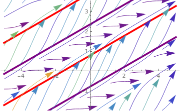
\frac{{\text d}y}{{\text d}x} = \cos \left( 2y-x \right) +1 , \qquad y(0) = \pi /4 .
\]
This problem can be solve at least implicitly by substitution:
z = 2
y - x , so
y = (
z+x )/2. Then for new dependent variable
z , we get a separable equation
\[
z' = 2y' -1 = 2\left( \cos z +1 \right) -1 = 2\,\cos z +1, \quad z(0) = \pi /2 .
\]
Separating variables and integrating, we obtain
\[
\frac{{\text d}z}{2\,\cos z + 1} = {\text d}x \qquad \Longrightarrow \qquad \frac{2}{\sqrt{3}}\,\mbox{arctanh} \left[ \frac{1}{\sqrt{3}}\,\tan \frac{z}{2} \right] = x +C,
\]
where
C is a constant of integration.
Integrate[1/(2*Cos[z] + 1), z]
(2 ArcTanh[Tan[z/2]/Sqrt[3]])/Sqrt[3]
Substitution the initial values into the relation yields
\[
\frac{1}{\sqrt{3}}\,\tan \frac{z}{2} = \tanh \left( C + \frac{\sqrt{3}}{2}\,x \right) \qquad \Longrightarrow \qquad C= \mbox{arctanh}\left( \frac{1}{\sqrt{3}} \right) \approx 0.6584789484624085.
\]
N[ArcTanh[1/Sqrt[3]]]
0.6584789484624085
So the implicit solution is
\[
\frac{1}{\sqrt{3}}\,\tan \frac{2y-x}{2} = \tanh \left( \mbox{arctanh}\left( \frac{1}{\sqrt{3}} \right) + \frac{\sqrt{3}}{2}\,x \right) .
\]
line1 = Plot[x/2 + Pi/4, {x, -5, 5},
PlotStyle -> {Red, Thickness[0.01]}];
Direction field along with separatrix lines.
Mathematica code
Now we use the modified decomposition method, assuming that the solution is represented by a convergent series
\[
y(x) = \sum_{n\ge 0} c_n x^n = \frac{\pi}{4} + \sum_{n\ge 1} c_n x^n .
\]
However, it is more convenient to find the Taylor series for the variable
z
\[
z(x) = \sum_{n\ge 0} b_n x^n = \frac{\pi}{2} + \sum_{n\ge 1} b_n x^n .
\]
Then the required coefficients will be
\[
c_n = \frac{1}{2}\, b_n + \frac{1}{2}\,\delta_{1,n} , \qquad n=0,1,2,\ldots ,
\]
where δ
1,n is the
Kronecker delta .
Indeed,
AsymptoticDSolveValue[{z'[x] == 2*Cos[z[x]] + 1, z[0] == Pi/2},
z[x], {x, 0, 6}]
\[
z(x) = \frac{\pi}{2} + x - x^2 + \frac{2\,x^3}{3} - \frac{x^4}{4} - \frac{x^5}{10} + \frac{37}{120}\,x^6 - \frac{7\,x^7}{20} + \frac{557\,x^8}{2240} + \frac{683\,x^9}{10080} + \cdots .
\qquad x\ne -1.
\]
We expand the solution into power series using the dedicated
Mathematica command:
AsymptoticDSolveValue[{y'[x] == Cos[2*y[x] - x] + 1, y[0] == Pi/4},
y[x], {x, 0, 6}]
\[
y(x) = \frac{\pi}{4} + x -\frac{x^2}{2} + \frac{x^3}{3} - \frac{x^4}{8} - \frac{x^5}{20} + \frac{37}{240}\,x^6 - \frac{7}{40}\, x^7 + \frac{557}{4480}\, x^8 - \frac{683}{20160}\, x^9 + \cdots .
\qquad x\ne -1.
\]
Substitution of Taylor series into the differential equation for
z , we obtain
\[
\sum_{n\ge 1} n\,b_n x^{n-1} = \sum_{n\ge 0} A_n \left( b_0, b_1 , \ldots , b_n \right) x^n +1,
\]
where
A n are the Adomian polynomials for the function
f (
z ) = 2 cos
z + 1:
\begin{align*}
A_0 &= f \left( b_0 \right) = f \left( \frac{\pi}{2} \right)= 2\,\cos \left( \frac{\pi}{2} \right) +1 = 1,
\\
A_1 &= b_1 f'\left( b_0 \right) = b_1 f'\left( \frac{\pi}{2} \right) = -2\,b_1 \sin \frac{\pi}{2} = -2\, b_1 ,
\\
A_2 &= b_2 f'\left( b_0 \right) + \frac{1}{2}\,b_1^2 f''\left( b_0 \right) = -2\, b_2 ,
\\
A_3 &= b_3 f'\left( b_0 \right) + \frac{1}{3!}\,b_1^3 f'''\left( b_0 \right) + b_1 b_2 f'\left( b_0 \right) = \frac{1}{3}\, b_1^3 -2\, b_3 ,
\\
A_4 &= b_1^2 b_2 -2\, b_1 b_3 ,
\\
A_5 &= - \frac{1}{60}\, b_1^5 + b_1 b_2^2 -2\, b_5 ,
\\
A_6 &= -\frac{1}{12}\,b_1^4 b_2 + \frac{1}{3}\,b_2^3 + 2\,b_1 b_2 b_3 + b_1^2 b_4 -2\, b_6 ,
\end{align*}
and so on. This allows us to derive the recurrence relation for coefficients {
b n }:
\begin{align*}
b_1 &= A_0 = 1,
\\
2\,b_2 &= A_1 = -2\, b_1 = -4 \qquad \Longrightarrow \qquad b_2 = -1 ,
\\
3\,b_3 &= A_2 = -2\, b_2 \qquad \Longrightarrow \qquad b_3 = - \frac{2}{3} ,
\end{align*}
Therefore, the power series solution becomes
\[
z(x) = \frac{\pi}{2} + x - x^2 - \frac{2}{3}\, x^3 - \frac{x^4}{4} - \frac{x^5}{10} + \frac{37}{120}\, x^6 + \cdots .
\]
s = ContourPlot[
1/Sqrt[3]*Tan[z/2] ==
Tanh[0.658478948462408 + x*Sqrt[3]/2], {x, -0.4, 4}, {z, 0, 2.1}]
Explicit solution and two polynomial approximations.
Mathematica code
■
Example: Rational slope function
Example:
\[
y' = \frac{3}{8}\, y - \frac{9t}{8\,y} , \qquad y(0) = 2.
\]
Since the given differential equation is a
Bernoulli one, its solution can be represented as the product
y (
t ) =
u (
t )
v (
t ), where
u (
t ) is a solution of the linear part of the Bernoulli equation
\[
u' = \frac{3}{8}\, u \qquad \Longrightarrow \qquad u(t) = e^{3\,t/8} .
\]
Another function
v (
t ) is the general solution of the separable equation
\[
u\,v' = - \frac{9t}{8\,u\,v} \qquad \Longrightarrow \qquad
v\,{\text d}v = - \frac{9t}{8\,u^2}\,{\text d}t = - \frac{9t}{8}\, e^{-3\,t/4}\,{\text d}t .
\]
Integration yields
Simplify[Integrate[-9*t/8*Exp[-3*t/4], t]]
\[
\frac{v^2}{2} = \frac{1}{2}\, e^{-3\,t/4} \left( 4+ 3\,t \right) + \frac{C}{2}
\qquad \Longrightarrow \qquad v^2 = e^{-3\,t/4} \left( 4+ 3\,t \right) + C ,
\]
where
C is a constant of integration. From the initial condition, it follows that
C = 0, and we get the explicit solution
\begin{align*}
y(t) &= \sqrt{4+3t}
\\
&= 2 + \frac{3}{4}\, t - \left( \frac{3\,t}{8} \right)^2 + \left( \frac{3\,t}{8} \right)^3 - \frac{5}{4} \left( \frac{3\,t}{8} \right)^4 + \frac{7}{4} \left( \frac{3\,t}{8} \right)^5 - \frac{21}{8} \left( \frac{3\,t}{8} \right)^6 + \frac{33}{8} \left( \frac{3\,t}{8} \right)^7 - \frac{429}{8^2} \left( \frac{3\,t}{8} \right)^8 + \cdots .
\end{align*}
Series[Sqrt[4 + 3*t], {t, 0, 8}]
We check with
Mathematica :
Series[Sqrt[4 + 3*t], {t, 0, 8}]
\[
2 + \frac{3\,t}{4} - \frac{9\,t^2}{64} + \frac{27\,t^3}{512} - \frac{405\,t^4}{16 384} + \frac{1701\,t^5}{131 072} - \frac{15309\, t^6}{2 097 152} + \frac{72171\, t^7}{16 777 216} - \frac{2814669\, t^8}{1 073 741 824} + \cdots .
\]
The same answe we obtain with another command
AsymptoticDSolveValue[{y'[t] == 3*y[t]/8 - 9*t/8/y[t], y[0] == 2},
y[t], {t, 0, 9}]
We determine this series using the MDM, so we assume that the solution is holomorphic in a neighbohood of the origin:
\[
y(t) = \sum_{n\ge 0} c_n t^n = 2 + \sum_{n\ge 1} c_n t^n .
\]
The Adomian polynomails corresponding to the reciprocal function
f (
y ) = 1/
y are
\begin{align*}
A_0 &= f \left( c_0 \right) = f \left( 2 \right) = \frac{1}{2} ,
\\
A_1 &= c_1 f'\left( c_0 \right) = - \frac{c_1}{c_0^2} = -\frac{c_1}{4} = - \frac{3}{16} ,
\\
A_2 &= c_2 f'\left( c_0 \right) + \frac{1}{2}\,c_1^2 f''\left( c_0 \right) = \frac{c_1^2}{c_0^3} -\frac{c_2}{c_0^2} = \frac{c_1^2}{8} -\frac{c_2}{4} ,
\\
A_3 &= c_3 f'\left( c_0 \right) + \frac{1}{3!}\,c_1^3 f'''\left( c_0 \right) + c_1 c_2 f'\left( c_0 \right) = -\frac{c_1^3}{c_0^4} + \frac{2\,c_1 c_2}{c_0^3} - \frac{c_3}{c_0^2} = -\frac{c_1^3}{16} + \frac{2\,c_1 c_2}{8} - \frac{c_3}{4} ,
\\
A_4 &= \frac{c_1^4}{c_0^5} - \frac{3\,c_1^2 c_2}{c_0^4} + \frac{c_2^2 + 2\,c_1 c_3}{c_0^3} - \frac{c_4}{c_0^2} ,
\\
A_5 &= - \frac{c_1^5}{c_0^6} + \frac{4\,c_1^3 c_2}{c_0^5} - \frac{3\,c_1 c_2^2 + 3\,c_1^2 c_3}{c_0^4} + \frac{2\,c_2 c_3 + 2\,c_1 c_4}{c_0^3} - \frac{c_5}{c_0^2} ,
\\
A_6 &= \frac{c_1^6}{c_0^7} - \frac{5\,c_1^4 c_2}{c_0^6} + \frac{6\,c_1^2 c_2^2 + 4\,c_1^3 c_3}{c_0^5} - \frac{c_2^3 + 6\,c_1 c_2 c_3 + 3\,c_1^2 c_4}{c_0^4} + \frac{c_3^2 + 2\,c_2 c_4 + 2\, c_1 c_5}{c_0^3} - \frac{c_6}{c_0^2} ,
\end{align*}
and so on. Substituting the power series into the given differential equation, we obtain
\[
\sum_{n\ge 1} n\,c_n t^{n-1} = \frac{3}{8}\, \sum_{n\ge 0} c_n t^n - \frac{9}{8}\,\sum_{n\ge 0} A_n t^{n+1} .
\]
Using the intial condition
y (0) =
c 0 = 2 and equating the coefficients of like powers, we get the recurrence relations:
\begin{align*}
c_1 &= \frac{3}{8}\, c_0 = \frac{3}{4} ,
\\
2\, c_2 &= \frac{3}{8}\, c_1 - \frac{9}{8}\,A_0 = - \frac{9}{32} \qquad \Longrightarrow \qquad c_2 = \frac{9}{64} ,
\\
3\,c_3 &= \frac{3}{8}\, c_2 - \frac{9}{8}\,A_1 = \frac{135}{512} \qquad \Longrightarrow \qquad c_3 = \frac{45}{512},
\\
4\, c_4 &= \frac{3}{8}\, c_3 - \frac{9}{8}\,A_2 =
\\
5\,c_5 &= \frac{3}{8}\, c_4 - \frac{9}{8}\,A_3 =
\\
6\,c_6 &= \frac{3}{8}\, c_5 - \frac{9}{8}\,A_4 =
\end{align*}
Explicit solution and two polynomial approximations.
s = Plot[Sqrt[4 + 3*t], {t, -0.5, 3}, PlotStyle -> Thick];
\( y(t) = \sqrt{4+3t} . \)
■
References
Adomian, G., Rach, R., Transformation of series, Applied Mathematics Letters
Volume 4, Issue 4, 1991, Pages 69-71; https://doi.org/10.1016/0893-9659(91)90058-4
Adomian, G., Rach, R., Nonlinear transformation of series—part II, Computers & Mathematics with Applications
Volume 23, Issue 10, May 1992, Pages 79-83; https://doi.org/10.1016/0898-1221(92)90058-P
Andrianov, I.V., Olevskii, V.I., Tokarzewski, S., A modified Adomian's decomposition method, Journal of Applied Mathematics and Mechanics , 1998, Volume 62, Issue 2, Pages 309--314; https://doi.org/10.1016/S0021-8928(98)00040-9
Bildik, N., Deniz, S., Modified Adomian decomposition method for solving Riccati differential equations , Review of the Air Force Academy , 2015, vol. 3, no. 30, pp. 21–26; doi: 10.19062/1842-9238.2015.13.3.3
Duan, J.-S. and Rach, R., The degenerate form of the Adomian polynomials in
the power series method for nonlinear ordinary differential equations ,
Journal of Mathematics and System Science , 2015, Volume 5, Pages 411--428, doi: 10.17265/2159-5291/2015.10.003
Duan, J.-S., Rach, R., New higher-order numerical one-step methods based on the Adomian and the modified decomposition methods, Applied Mathematics and Computation , 2011, Vol. 218, pp. 2810--2828.
Duan, J.-S., Rach, R., Wazwaz, A.-M., Solution of the model of beam-type
micro- and nano-scale electrostatic actuators by a new modified
Adomian decomposition method for nonlinear boundary value problems,
International Journal of Non-Linear Mechanics , 2013, Volume 49, 2013, Pages
159--169.
Rach, R., Adomian, G., Meyers, R., A modified decomposition method, Computers & Mathematics with Applications , 1992,
Volume 23, Issue 1, January 1992, Pages 17-23; https://doi.org/10.1016/0898-1221(92)90076-T
Return to Mathematica page main page (APMA0330) Part 1 (Plotting)Part 2 (First Order ODEs)Part 3 (Numerical Methods)Part 4 (Second and Higher Order ODEs)Part 5 (Series and Recurrences) Part 6 (Laplace Transform) Part 7 (Boundary Value Problems)