Preface

This section addresses an introduction to the fascinating topic that originated in the work of the American mathematician and meteorologist Edward Norton Lorenz (1917--2008). He discovered what is known now as deterministic chaos in mathematics and physics. The deterministic nature of dynamic systems does not make them predictable (determined) in practice. Solutions of differential systems involving more than two nonlinear differential equations may be qualitatively different from the planar solutions since slight perturbation may leads to exponential deviation. The idea was summarized by Edward Lorenz as: Chaos – when the present determines the future, but the approximate present does not approximately determine the future.

The history of Lorenz discovery can be found in James Gleick's (born 1954) book. Gleick, formerly a science writer for the New York Times, depicts the beginnings of Chaos theory, which draws on the seemingly random patterns that characterize many natural phenomena. It explains the thought processes and investigative techniques of Chaos scientists, illustrating concepts like Julia sets, Lorenz attractors, and the Mandelbrot Set with sketches, photographs, and wonderfully descriptive prose. This highly readable international best-seller is must-reading for any Clausewitzian. (See Alan D. Beyerchen's essay on the connection with Clausewitz. ISBN: 0143113453.)

Lorenz equations

An important problem in meteorology and in other applications of fluid dynamics is modeling a layer of fluid such as the earth's atmosphere. (Lorenz's derivation (1963) was based on considering a two-dimensional fluid cell (or layer) that is warmed from below and cooled from above. If the vertical temperature difference ΔT is small, then there is a linear variation of temperature with altitude, but no significant motion of the fluid layer. However, if ΔT is large enough, then the warmer air rises, displacing the cooler air above it, and steady convective motion results. If the temperature difference increases further, then eventually the steady convective flow breaks up and a more complex and turbulent motion ensues. Edward Lorenz was led to the nonlinear autonomous dynamic system:

Edward Lorenz was born in West Hartford, Connecticut. He studied mathematics at both Dartmouth College in New Hampshire and Harvard University in Cambridge, Massachusetts. From 1942 until 1946, he served as a meteorologist for the United States Army Air Corps. After his return from World War II, he decided to study meteorology. Lorenz earned two degrees in the area from the Massachusetts Institute of Technology. Dr. Lorenz was a staff member of the MIT meteorology department from 1948 to 1955, when he became an assistant professor. He was promoted to professor in 1962 and served as head of the department from 1977 to 1981. During the 1950s, Lorenz became skeptical of the appropriateness of the linear statistical models in meteorology, as most atmospheric phenomena involved in weather forecasting are non-linear. His work on the topic culminated in the publication of his 1963 paper "Deterministic Nonperiodic Flow" in Journal of the Atmospheric Sciences, and with it, the foundation of chaos theory. He was awarded the Kyoto Prize for basic sciences, in the field of earth and planetary sciences, in 1991.

Dr. Lorenz is best known for the notion (in 1969) of the “butterfly effect,” the idea that a small disturbance like the flapping of a butterfly’s wings can induce enormous consequences. His chaos discovery was accidental. One day, Dr. Lorenz was running simulations of weather using a simple computer model. Another day, he wanted to repeat one of the simulations for a longer time, but instead of repeating the whole simulation, he started the second run in the middle, typing in numbers from the first run for the initial conditions. The computer program was the same, so the weather patterns of the second run should have exactly followed those of the first. Instead, the two weather trajectories quickly diverged on completely separate paths.

At first, he thought the computer was malfunctioning. Then he realized that he had not entered the initial conditions exactly. The computer stored numbers to an accuracy of six decimal places, like 0.506127, while, to save space, the printout of results shortened the numbers to three decimal places, 0.506. When typing in the new conditions, Dr. Lorenz had entered the rounded-off numbers, and even this small discrepancy, of less than 0.1 percent, completely changed the final result. Even though his model was vastly simplified, Dr. Lorenz realized that this meant perfect weather prediction was a fantasy. A perfect forecast would require not only a perfect model, but also perfect knowledge of wind, temperature, humidity and other conditions everywhere around the world at one moment of time. Even a small discrepancy could lead to completely different weather. In 1972, he gave a talk with a title that captured the essence of his ideas: “Predictability: Does the Flap of a Butterfly’s Wings in Brazil Set Off a Tornado in Texas?”

In his later years, Lorenz lived in Cambridge, Massachusetts. He was an avid outdoors man, who enjoyed hiking, climbing, and cross-country skiing. He kept up with these pursuits until very late in his life, and managed to continue most of his regular activities until only a few weeks before his death. According to his daughter, Cheryl Lorenz, Lorenz had "finished a paper a week ago with a colleague." On April 16, 2008, Lorenz died at his home in Cambridge at the age of 90, having suffered from cancer.

The Lorenz equations are made up of three populations: x, y, and z, and three fixed coefficients: σ, ρ, and β. Remembering what we discussed previously, this system of equations has properties common to most other complex systems, such as lasers, dynamos, thermosiphons, brushless DC motors, electronic circuits, and chemical reactions. First, it is non-linear in two places: the second equation has an xz term and the third equation has an xy term. It is made up of a very few simple components. The system is three-dimensional and deterministic. Although difficult to see until we plot the solution, the equation displays broken symmetry on multiple scales. Because the equation is autonomous (no t term in the right side of the equations), there is no feedback in this case.

Example 1: We consider the Lorenz's equations under the following values of parameters:

\[ \sigma = 10, \quad \beta = 8/3, \rho = 28. \]

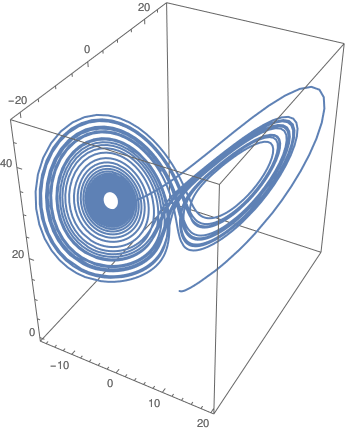
		\[Sigma] = 10; solution = NDSolve[{x'[t] == \[Sigma] (y[t] - x[t]), y'[t] == 28 x[t] - y[t] - x[t] z[t], z'[t] == x[t] y[t] - 8/3 z[t], x[0] == z[0] == 0, y[0] == 2}, {x, y, z}, {t, 0, 35}] ParametricPlot3D[Evaluate[{x[t], y[t], z[t]} /. solution], {t, 0, 35}]
Lorenz attractor.		Mathematica code

   ■

End of Example 1

Example 2: We seek solutions of the Lorenz equations as power series

\begin{align*} x(t) &= \sum_{i\ge 0} \frac{a_i}{i!}\left( t - t_0 \right)^i , \\ y(t) &= \sum_{k\ge 0} \frac{b_k}{k!} \left( t - t_0 \right)^k , \\ z(t) &= \sum_{m\ge 0} \frac{c_m}{k!} \left( t - t_0 \right)^m \end{align*}

upon substituting into the system of equations. This yields the following recurrence:

\begin{align*} a_k &= - \sigma \,a_{k-1} + \sigma\,b_{k-1} , \qquad k \ge 1, \quad a_0 = x(t_0 ) , \\ b_{k+1} &= r\,a_k - b_k - k! \,\sum_{i=0}^k \frac{a_i \,c_{k-i}}{i!\,(k-i)!} , \qquad k \ge 0, \quad b_0 = y(t_0 ) , \\ c_{k+1} &= b\, c_k + k! \,\sum_{i=0}^k \frac{a_i \,b_{k-i}}{i!\,(k-i)!} , \qquad k \ge 0, \quad c_0 = z(t_0 ) \end{align*}

Module[ { a, b, c, \[Sigma], \[Rho] , \[Beta] , x, y, z, k }, x[t0] = 0; y[t0] = 0; z[t0] = 0; RecurrenceTable[ { a[k] == \[Sigma] a[k - 1] + \[Sigma] b[k - 1] , b[k + 1] == \[Rho] a[k] - b[k] - k! Sum[a[i] c[k - i]/(i! (k - i)!), {i, 0, k}], c[k + 1] == \[Beta] c[k] - k! Sum[a[i] b[k - i]/(i! (k - i)!), {i, 0, k}], a[0] == x[t0], b[0] == y[t0], c[0] == z[t0] }, {a, b, c}, {k, 1, 20} ] ];

Evaluating the recurrence equations below at k = 1 shows that the values of b[1] and c[1] are unknown:

{ a[k] == \[Sigma] a[k - 1] + \[Sigma] b[k - 1] , b[k + 1] == \[Rho] a[k] - b[k] - k! Sum[a[i] c[k - i]/(i! (k - i)!), {i, 0, k}], c[k + 1] == \[Beta] c[k] - k! Sum[a[i] b[k - i]/(i! (k - i)!), {i, 0, k}], a[0] == x[t0], b[0] == y[t0], c[0] == z[t0] } /. k -> 1 // TableForm

Clear[x, y, z, a, b, c, i, k, m, t, t0] (* Define the power series *) x[t_, t0_, a_] := Sum[a[i]/i! (t - t0)^i, {i, 0, Infinity}] y[t_, t0_, b_] := Sum[b[k]/k! (t - t0)^k, {k, 0, Infinity}] z[t_, t0_, c_] := Sum[c[m]/m! (t - t0)^m, {m, 0, Infinity}]

Define the recurrence relations

a[k_, \[Sigma]_, a_, b_] := -\[Sigma] a[k - 1] + \[Sigma] b[k - 1] /; k >= 1 b[k_ + 1, r_, a_, b_, c_] := r a[k] - b[k] - k! Sum[a[i] c[k - i]/(i! (k - i)!), {i, 0, k}] /; k >= 0 c[k_ + 1, b_, c_] := b c[k] + k! Sum[a[i] b[k - i]/(i! (k - i)!), {i, 0, k}] /; k >= 0

Set initial conditions

a[0] = x[t0]; b[0] = y[t0]; c[0] = z[t0];

Visualize the equations

Grid[{ {"x(t)", x[t, t0, a]}, {"y(t)", y[t, t0, b]}, {"z(t)", z[t, t0, c]}, {"Recurrence for a_k", a[k, \[Sigma], a, b]}, {"Recurrence for b_(k+1)", b[k + 1, r, a, b, c]}, {"Recurrence for c_(k+1)", c[k + 1, b, c]} }, Frame -> All]

Define parameters

\[Sigma] = 10; r = 28; b = 8/3; t0 = 0;

Number of terms in the series

numTerms = 5;

Initialize coefficient lists

aCoeffs = ConstantArray[0, numTerms + 1]; bCoeffs = ConstantArray[0, numTerms + 1]; cCoeffs = ConstantArray[0, numTerms + 1];

Set initial conditions

aCoeffs[[1]] = 1; (* Corresponds to a[0] *) bCoeffs[[1]] = 1; (* Corresponds to b[0] *) cCoeffs[[1]] = 1; (* Corresponds to c[0] *)

Compute coefficients using recurrence relations

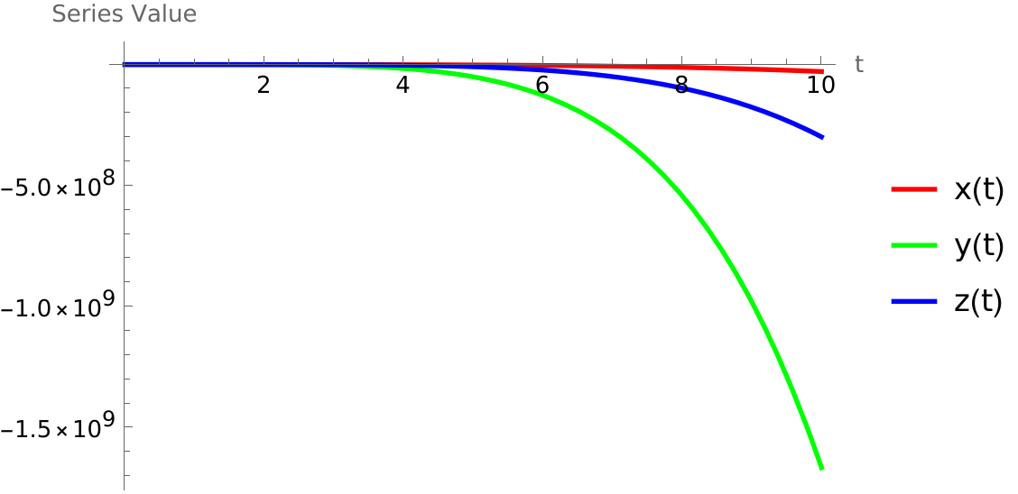
Do[ aCoeffs[[ k + 1]] = -\[Sigma] aCoeffs[[k]] + \[Sigma] bCoeffs[[k]]; bCoeffs[[k + 2]] = r aCoeffs[[k + 1]] - bCoeffs[[k + 1]] - k! Sum[ aCoeffs[[i + 1]] cCoeffs[[k - i + 1]]/(i! (k - i)!), {i, 0, k}]; cCoeffs[[k + 2]] = b cCoeffs[[k + 1]] + k! Sum[ aCoeffs[[i + 1]] bCoeffs[[k - i + 1]]/(i! (k - i)!), {i, 0, k}]; , {k, 0, numTerms - 1}]; (* Define the series *) xSeries[t_] := Sum[aCoeffs[[i + 1]]/i! (t - t0)^i, {i, 0, numTerms}] ySeries[t_] := Sum[bCoeffs[[k + 1]]/k! (t - t0)^k, {k, 0, numTerms}] zSeries[t_] := Sum[cCoeffs[[m + 1]]/m! (t - t0)^m, {m, 0, numTerms}] (* Plot the series *) Plot[{xSeries[t], ySeries[t], zSeries[t]}, {t, t0, 1}, PlotLegends -> {"x(t)", "y(t)", "z(t)"}, PlotStyle -> {Red, Green, Blue}, AxesLabel -> {"t", "Series Value"}, PlotRange -> All]

   ■

End of Example 2

Example 3: The Glukhovsky--Dolzhanksy system is of the following form:

\[ \begin{split} \dot{x} = -\sigma \left( x - y \right) -a yz , \\ \dot{y} = rx - y -xz , \\ \dot{z} = - bz + xy , \end{split} \]

where σ, 𝑎, r, b are physical parameters. Comparing this to the well-known Lorenz system, it has an additional non-linear term, which leads to essential differences in analytical structure and dynamics of the system. The Glukhovsky--Dolzhansky system describes the following physical processes: convective fluid motion in an ellipsoidal rotating cavity, a rigid body rotation in a resisting medium, the forced motion of a gyrostat, a convective motion in harmonically oscillating horizontal fluid layer. Initially, this system was obtained by Glukhovsky and Dolzhansky as a three-mode model of convection for a fluid in an ellipsoidal rotating cavity, which can be interpreted as one of the models of ocean flows.

		Here is Mathematica code for plotting Glukhovsky-Dolzhansky system: \[Sigma] = 10; a = 0; r = 24; b = 8/3; s = NDSolve[{x'[t] == -\[Sigma]*(x[t] - y[t]) - a*(y[t]*z[t]), y'[t] == r*x[t] - y[t] - x[t]*z[t], z'[t] == -b*z[t] + x[t]*y[t], x[0] == z[0] == 0, y[0] == 2}, {x, y, z}, {t, 0, 100}]; ParametricPlot3D[Evaluate[{x[t], y[t], z[t]} /. s], {t, 0, 70}, PlotTheme -> "Business"]
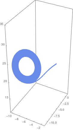
Solution of Glukhovsky-Dolzhansky system.		Mathematica code

Here is a subroutine for solving the Glukhovsky-Dolzhansky (GD for short) system:

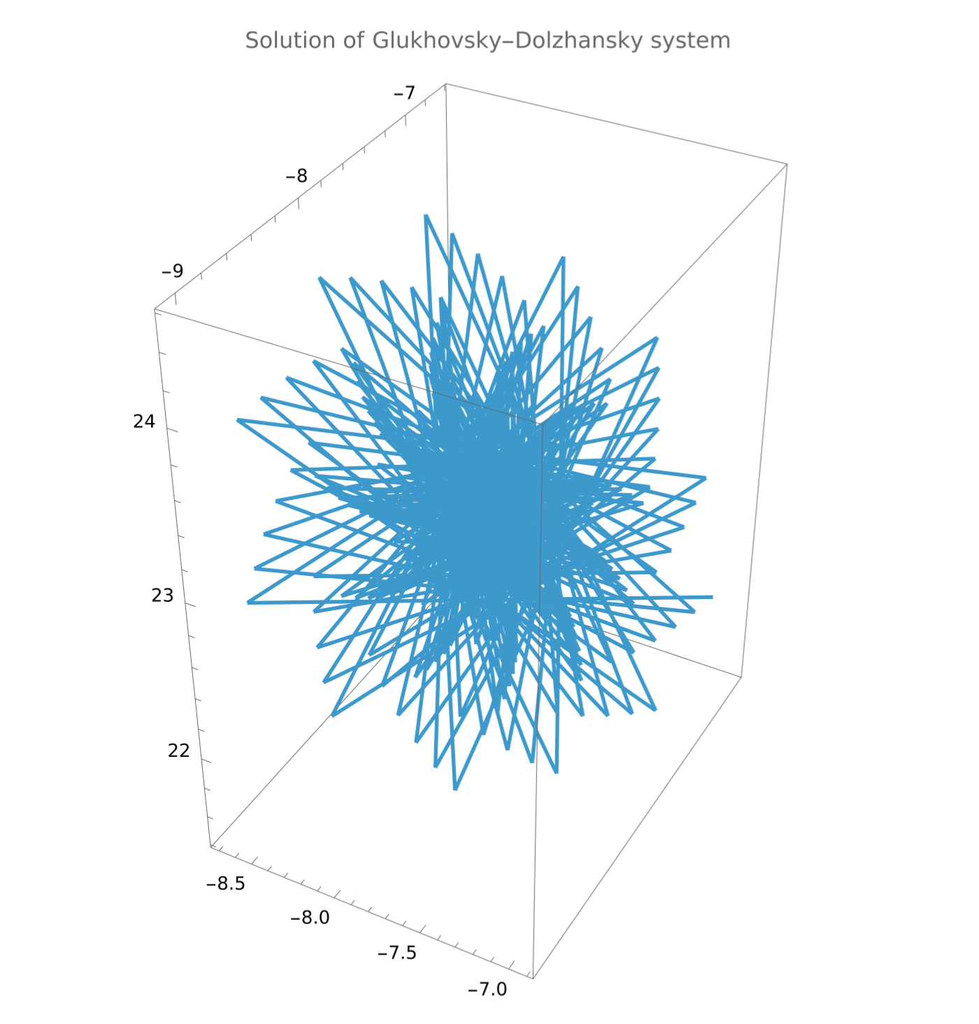
lorMod = Module[ { \[Sigma] = 10, a = 0, r = 24, b = 8/3, tStart = 0, tEnd = 1000 }, {x[t], y[t], z[t]} /. NDSolve[ { x'[t] == -\[Sigma] (x[t] - y[t]) - a (y[t] z[t]), y'[t] == r x[t] - y[t] - x[t] z[t], z'[t] == -b z[t] + x[t] y[t], x[0] == 0, z[0] == 0, y[0] == 2 }, {x, y, z}, {t, tStart, tEnd} ] ]; Manipulate[ ParametricPlot3D[ Evaluate@lorMod, {t, tMin, tMax}, PlotRange -> All, PlotLabel -> "Solution of Glukhovsky-Dolzhansky system", ImageSize -> 500 ], {tMin, 0, 999}, {tMax, 1, 1000}, ContinuousAction -> False ]

   ■

End of Example 3

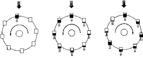
Example 5: A neat mechanical model of the Lorenz equations was invented by Willem Malkus and Lou Howard at MIT (Cambridge, MA, USA) in the 1970s. A Lorenzian (or "chaotic") waterwheel is a physical model that perfectly corresponds to the Lorenz equations. A chaotic waterwheel is just like a normal waterwheel except for the facts that the buckets leak. Water pours into the top bucket at a steady rate and gives the system energy while water leaks out of each bucket at a steady rate and removes energy from the system. If the parameters of the wheel are set correctly, the wheel will exhibit chaotic motion: rather than spinning in one direction at a constant speed, the wheel will speed up, slow down, stop, change directions, and oscillate back and forth between combinations of behaviors in an unpredictable manner. Its derivation is given in Strogatz's book Nonlinear Dynamics and Chaos, section 9.1:

\[ \begin{split} \dot{a} = omega\,b - K\,a, \\ \dot{b} = -\omega\,a -K\,b + q , \\ \dot{\omega} = -\frac{\nu}{I}\,\omega + \frac{\pi G\,r}{I}\, a , \end{split} \]

where
I is the moment of inertia of the wheel,
θ is the angle of the wheel,
\( \omega = \dot{\theta} \) is the angular velocity (increases counterclockwise, as does θ),
K is is the liquid’s leakage rate,
ν is the rotational damping rate,
r is the radius of the wheel,
G is the effective gravity constant.

The dependent variables 𝑎 = 𝑎₁ and b = b₁ are the Fourier amplitudes of the first modes of the liquid's mass distribution function of water around the rim of the wheel, defined such that the mass between θ₁ and θ₂ is \( M(t) = \int_{\theta_1}^{\theta_2} m(\theta , t)\,{\text d}\theta , \)

\[ m(\theta , t ) = \sum_{n\ge 0} a_n (t)\,\cos n\theta + b_n \sin n\theta . \]

Here q = q₁ is the Fourier amplitude of the first mode of the liquid inflow mass distribution function

\[ Q(\theta ) = \sum_{n\ge 0} q_n \cos nm\theta . \]

So Q(θ) is the inflow (rate at which water is pumped in by the nozzles above position θ.

Lorenz, E.N. The Essence of Chaos, 1 ed.; University of Washington Press: Seattle, DA, USA, 1993; pp. 1–227. https://doi.org/10.1 201/97814822889887.

Illing, L.; Fordyce, R.F.; Saunders, A.M.; Ormond, R. Experiments with a Malkus–Lorenz water wheel: Chaos and synchronization. Am. J. Phys. 2012, 80, 192–202. https://doi.org/10.1119/1.3680533.

Tongen, A.; Thelwell, R.J.; Becerra-Alonso, D. Reinventing the wheel: The chaotic sandwheel. Am. J. Phys. 2013, 81, 127–133. https://doi.org/10.1119/1.4768893.    ■

End of Example 5

In this short-term financial model, which is a model for short-term interest rate, it is intended to give a natural explanation of the behavior of this economic variable. Let us consider the dynamics of an interest rate model in the short term, in the following general form of Equation

Furthermore, there are several studies in which the short-rate behavior is explained by monetary policy (monetary flow (see Dornbusch)).

The IS-LM model (here IS stands for "investment-saving" and LM is "Liquidity-money"), like any other in economics, is represented by equations in equilibrium. In this case, there are two state variables X = (r, y), where r is the short real rate and y is the real national income rate. The two corresponding equilibrium ratios are: the money supply plus the monetary demand m_d, and the real national income rate and the real national expenditure rate e. Values m_d and e are related to r and y by equations

This last equation has been rewritten in such a way that it is a function of x and r, as it is necessary to determine the behavior of r as a function of x, in which r is fed back to x. Here, x represents the expected value of the interest rate. The process of x implicitly explains the economy.

If α = v and β = α_y (1 − c) is defined, then the previous equations can be written as Equation

In this two-factor model, p represents the r-influence on the expected level of the interest rate x. It measures the degree of feedback between r and the rest of the economy. In this system p is constant, however, in practice the parameter values, and therefore p, are determined by the aggregated behavior of the individuals involved in the economy. If the p-dynamics to the system is added in Equation (24) (a three-factor model), then we can define \[ {\text d}p = \gamma \left( \overline{p} - p \right) {\text d}t + \sigma_p {\text d}z_p , \] where the equilibrium value of p is \( \displaystyle \quad \overline{p} \quad \) and γ is the feedback rate from p to \( \displaystyle \quad \overline{p} \quad \) .

The complete three-factor system is expressed as follows:

The nature of the system is clarified by introducing a change in variables, assuming that the system is not volatile i.e., that the model is deterministic as \[ X = \frac{r-\mu}{s} , \quad Y = \frac{x-\mu}{s}\,y , \quad Z = \delta - p , \] where \( \displaystyle \quad s = \sqrt{1/\gamma \phi} . \quad \) With the assumption of zero volatility and with this definition of parameters, a system can be obtained, which is equivalent to that of Lorenz in Equation

Tice, J.; Webber, N. A Nonlinear Model of the Term Structure of Interest Rates 1997. 7, 177–209. https://doi.org/10.1111/1467-9 965.00030.

Dornbusch, R.; Fischer, S.; Startz, R. Macroeconomics, 11 ed.; McGraw-Hill: New York, USA, 2011; pp. 248–271.

Haag, G.; Hagel, T.; Sigg, T. Active stabilization of a chaotic urban system. Discrete Dyn. Nat. Soc. 1997, 1, 127–134. https://doi.org/10.1155/S1026022697000137.518    ■