Preface


This section studies some first order nonlinear ordinary differential equations describing the time evolution (or “motion”) of those hamiltonian systems provided with a first integral linking implicitly both variables to a motion constant. An application has been performed on the Lotka--Volterra predator-prey system, turning to a strongly nonlinear differential equation in the phase variables.

Return to computing page for the first course APMA0330
Return to computing page for the second course APMA0340
Return to Mathematica tutorial for the first course APMA0330
Return to Mathematica tutorial for the second course APMA0340
Return to the main page for the first course APMA0330
Return to the main page for the second course APMA0340
Return to Part III of the course APMA0340
Introduction to Linear Algebra with Mathematica

Pendulum numerical simulation


Example: We use Mathematica:
fx = Function[{x, y}, y]; fy = Function[{x, y}, -Sin[x] - 0.25*y]
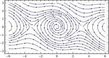
portrait =
StreamPlot[{fx[x, y], fy[x, y]}, {x, -6, 6}, {y, -3, 3},
AspectRatio -> Automatic]
solution =
Function[point, Function @@ {t, ({x[t], y[t]} /.
NDSolve[{x'[t] == fx[x[t], y[t]], y'[t] == fy[x[t], y[t]],
Thred[{x[time], y[time]} == point]}, {x, y}, {t, time,
time + 40}])[[1]]}]
Out[12]=
Function[point, Function @@ {t, ({x[t], y[t]} /.
NDSolve[{Derivative[1][x][t] == fx[x[t], y[t]],
Derivative[1][y][t] == fy[x[t], y[t]],
Thred[{x[time], y[time]} == point]}, {x, y}, {t, time, time + 40}])[[1]]}]
To numerically solve the pendulum equation, we first define the system:
osc[gamma_, omega_, x0_, v0_] := {x'[t] == v[t], v'[t] == -gamma*v[t] - omega^2*Sin[x[t]], x[0] == x0, v[0] == v0}
Then, we define a routine which gives the result of integrating the differential equation with NDSolve, starting at t = 0, and integrating out to t = tfinal.
ans[gamma_, omega_, x0_, v0_, tfinal_] := {x[t], v[t]} /. Flatten[NDSolve[ osc[gamma, omega, x0, v0], {x[t], v[t]}, {t, 0, tfinal}]]
We try this out:
sol1 = ans[0.25, 1, 1, 0, 10]
Out[8]= = {InterpolatingFunction[{{0., 10.}}, <>][t], InterpolatingFunction[{{0., 10.}}, <>][t]}
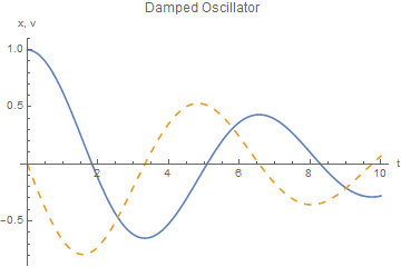
The output sol1 contains the two interpolating functions (Mathematica uses cubic splines) that represent x(t) and v(t). We can evaluate them or plot them. For example, the values at t = 3 are
sol1 /. t -> 3
Out[11]= {-0.6186, -0.201005}
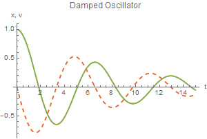
We now plot x and v as functions of t, using solid for x and dashed for v.
graph1 = Plot[{First[sol1], Last[sol1]}, {t, 0, 10}, AxesLabel -> {"t", "x, v"}, PlotLabel -> "Damped Oscillator",
PlotStyle -> {Dashing[{}], Dashing[{0.02, 0.02}]}]
Now we assign separate names to the x(t) and y(t) components of the solution
xsol1[t_] := First[sol1]
ysol1[t_] := Last[sol1]
Then we can reproduce the above graph:
graph2 = Plot[{sol1, sol1}, {t, 0, 15}, AxesLabel -> {"t", "x, v"}, PlotLabel -> "Damped Oscillator", PlotStyle -> {Dashing[{}], Dashing[{0.02, 0.02}]}]
Now we do something new by plotting y versus x:
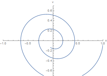
graph3 = ParametricPlot[{xsol1[t], ysol1[t]}, {t, 0, 15}, PlotRange -> {{-1, 1}, {-0.7, 0.7}}, AxesLabel -> {"x", "v"}]
For this underdamped oscillator, we see that the phase plot is a spiral. As time increases, the system point moves inward towards the equilibrium at x = 0, v = 0. In physical terms, the oscillations decrease in amplitude as the damping takes energy out of the system.

We could also construct the plot without referring separately to sol1 contains the two interpolating functions (Mathematica uses cubic splines) that represent x(t) and v(t). We can evaluate them or plot them. For example, the values at t = 3 are
sol1 /. t -> 3
Out[11]= {-0.6186, -0.201005}
We now plot x and v as functions of t, using solid for x and dashed for v.
graph1 = Plot[{First[sol1], Last[sol1]}, {t, 0, 10}, AxesLabel -> {"t", "x, v"}, PlotLabel -> "Damped Oscillator",
PlotStyle -> {Dashing[{}], Dashing[{0.02, 0.02}]}]
Now we assign separate names to the x(t) and y(t) components of the solution
xsol1[t_] := First[sol1]
ysol1[t_] := Last[sol1]
Then we can reproduce the above graph:
graph2 = Plot[{sol1, sol1}, {t, 0, 15}, AxesLabel -> {"t", "x, v"}, PlotLabel -> "Damped Oscillator", PlotStyle -> {Dashing[{}], Dashing[{0.02, 0.02}]}]
Now we do something new by plotting y versus x:
graph3 = ParametricPlot[{xsol1[t], ysol1[t]}, {t, 0, 15}, PlotRange -> {{-1, 1}, {-0.7, 0.7}}, AxesLabel -> {"x", "v"}]
For this underdamped oscillator, we see that the phase plot is a spiral. As time increases, the system point moves inward towards the equilibrium at x = 0, v = 0. In physical terms, the oscillations decrease in amplitude as the damping takes energy out of the system.

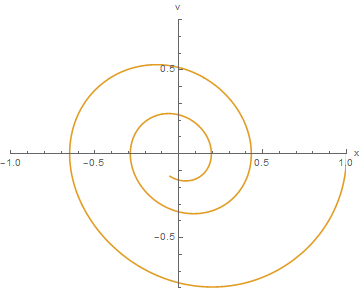
We could also construct the plot without referring separately to xsol1 and ysol1.
graph4 = ParametricPlot[sol1, {t, 0, 15}, PlotRange -> {{-1, 1}, {-0.8, 0.8}}, AxesLabel -> {"x", "v"}]

Now we turn to plotting solutions of the pendulum equation subject to distinct initial conditions. Actually, we define three solutions:

sol2 = ans[0.25, 1, 2, 0, 15]
sol3 = ans[0.25, 1, 3, 0, 15]
Now we plot them.
ParametricPlot[{{First[sol1], Last[sol1]}, {First[sol2], Last[sol2]}, {First[sol3], Last[sol3]}}, {t, 0, 15},
PlotRange -> {{-1.6, 3.1}, {-1.9, 1.4}}, AxesLabel -> {"x", "v"}, PlotStyle -> {{Thick, Red}, {Thick, Blue}, {Thick, Green}}]
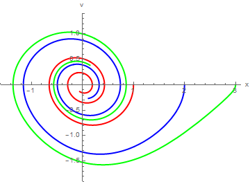
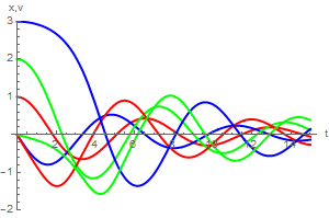
Every solution of this equation spirals in toward the equilibrium point at {0,0}. None of these spirals intersect other spirals, and none intersects itself. The phase plane provides an excellent way to visualize such a family of solutions. If we attempt to view these solutions simultaneously as functions of t, the result is quite cluttered:
Plot[{First[sol1], Last[sol1], First[sol2], Last[sol2], First[sol3], Last[sol3]}, {t, 0, 15}, AxesLabel -> {"t", "x,v"},
PlotRange -> {-2, 3}, PlotStyle -> {{Thick, Red}, {Thick, Blue}, {Thick, Green}}]
 

Return to Mathematica page
Return to the main page (APMA0340)
Return to the Part 1 Matrix Algebra
Return to the Part 2 Linear Systems of Ordinary Differential Equations
Return to the Part 3 Non-linear Systems of Ordinary Differential Equations
Return to the Part 4 Numerical Methods
Return to the Part 5 Fourier Series
Return to the Part 6 Partial Differential Equations
Return to the Part 7 Special Functions