Return to computing page for the first course APMA0330
Return to computing page for the second course APMA0340
Return to Mathematica tutorial for the first course APMA0330
Return to Mathematica tutorial for the second course APMA0340
Return to the main page for the first course APMA0330
Return to the main page for the second course APMA0340
Return to Part VI of the course APMA0340
Introduction to Linear Algebra with Mathematica
Glossary
Applications
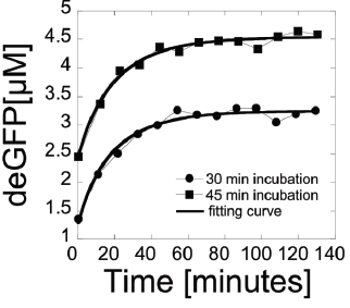
Example 1: A balance between protein and mRNA synthesis and degredation/inactivation can be modeled to help in laboratory testing of processes involving biological information. A certain study uses an E. coli cell-free expression system, where the informational elements (mRNA and proteins) are studied outside of the body and their respective cells. Testing processes in these conditions is key to developing new biological engineering applications.
In this example, we examine endogenous mRNA inactivation to better understand gene expression dynamics. The protein used is deGFP, which is a highly translatable green fluorescent protein. The following differential equations describe the rate of change over time of the concentration of deGFP mRNA (m), dark deGFP (deGFPd), and fluorescent deGFP (deGFPf).
clear;
syms B m(t) deGFPd(t) a k deGFPf(t);
eqns=[diff(m)==-B*m;diff(deGFPd)==a*m-k*deGFPd;diff(deGFPf)==k*deGFPd]
The various constants are defined as the protein production rate a, the mRNA inactivation rate B, and the maturation time of the protein 1/k (including folding, etc). The following initial conditions are given in the study as the starting point for the respective assays:
cond=[deGFPf(0)==0;deGFPd(0)==0.25;m(0)==0.25]We solve the above differential equations using these initial conditions to find equations for the concentration of each item in terms of time.
soln=dsolve([eqns;cond]);
deGFPd_(t)=soln.deGFPd
m_(t)=soln.m
deGFPf_(t)=soln.deGFPf
Example 2: The differential equation governing the motion of a particle with electric charge q in an electromagnetic field is
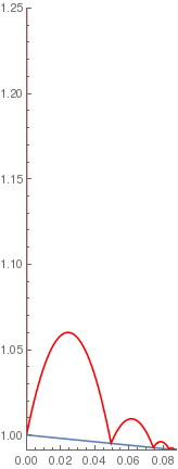
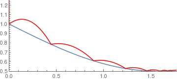
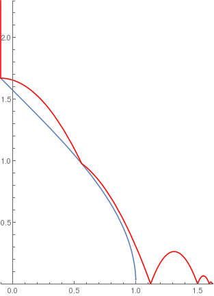
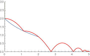
Example 3: Suppose that a ball of mass m is released with some initial velocity from a particular point over a surface. Then its position (x,y) is determined from the follwoing initial avlue problem
(*Calculates the position and velocity of the ball after one bounce \ on a given curve*)
Module[{sol, t1, x1, xp1, y1, yp1, gramp, gp},
sol = First[ NDSolve[{x''[t] == 0, x'[t0] == xp0, x[t0] == x0, y''[t] == -9.8,
y'[t0] == yp0, y[t0] == y0}, {x, y}, {t, t0, Infinity},
Method -> {"EventLocator", "Event" :> y[t] - ramp[x[t]]},
MaxStepSize -> 0.01]];
t1 = InterpolatingFunctionDomain[x /. sol][[1, -1]];
{x1, xp1, y1, yp1} = Reflection[k, ramp][{x[t1], x'[t1], y[t1], y'[t1]} /. sol];
Sow[{x[t] /. sol, t0 <= t <= t1}, "X"];
Sow[{y[t] /. sol, t0 <= t <= t1}, "Y"];
Sow[{x1, y1}, "Bounces"];
{t1, x1, xp1, y1, yp1}]
(*Calculates the position and velocity of the ball after reflecting \ off of the curve*)
Module[{gramp, gp, xpnew, ypnew}, gramp = -ramp'[x];
If[Not[NumberQ[gramp]], Print["Could not compute derivative"];
Throw[$Failed]];
gramp = {-ramp'[x], 1};
If[gramp.{xp, yp} == 0, Print["No reflection"];
Throw[$Failed]];
gp = {1, -1} Reverse[gramp];
{xpnew, ypnew} = (k/(gramp.gramp)) (gp gp.{xp, yp} - gramp gramp.{xp, yp});
{x, xpnew, y, ypnew}]
(*Calculates the path of the ball over a specific range of x bounce \ by bounce and plots it*)
Module[{data, end, bounces, xmin, xmax, ymin, ymax}, If[y0 < ramp[x0], Print["Start above the ramp"];
Return[$Failed]];
data = Reap[Catch[Sow[{x0, y0}, "Bounces"];
NestWhile[OneBounce[k, ramp], {0, x0, 0, y0, 0}, Function[1 - #1[[1]] / #2[[1]] > 0.01], 2, 25]], _, Rule];
end = data[[1, 1]];
data = Last[data];
bounces = ("Bounces" /. data);
xmax = Max[bounces[[All, 1]]];
xmin = Min[bounces[[All, 1]]];
ymax = Max[bounces[[All, 2]]];
ymin = Min[bounces[[All, 2]]];
Show[{Plot[ramp[x], {x, xmin, xmax}, PlotRange -> {{xmin, xmax}, {ymin, ymax}}, AspectRatio -> (ymax - ymin) / (xmax - xmin)],
ParametricPlot[ Evaluate[{Piecewise["X" /. data], Piecewise["Y" /. data]}], {t, 0, end}, PlotStyle -> RGBColor[1, 0, 0]]}]]
|
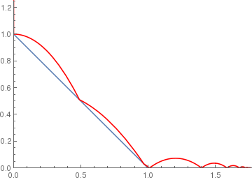
ramp[x_] := If[x < 1, 1 - x, 0];
BouncingBall[.7, ramp, {0, 1.25}] |
 |
|
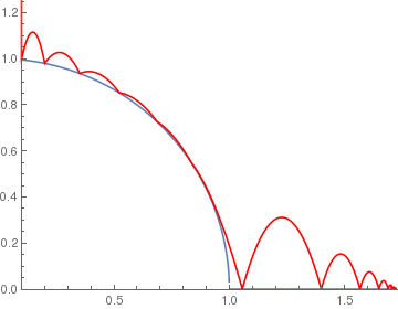
(* 0.7 means the coefficient of rebouncing *)
circle[x_] := If[x < 1, Sqrt[1 - x^2], 0]; BouncingBall[.7, circle, {.1, 1.25}] |
 |
|
|
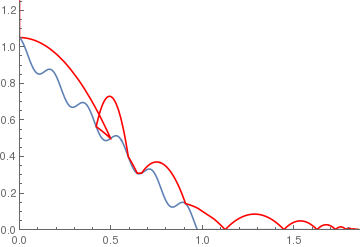
wavyramp[x_] := If[x < 1, 1 - x + .05 Cos[11 Pi*x], 0];
 |
|
|
(*Small slope linear with high friction*)
 |
|
(*Sine wave ramp*)
sineramp[x_] := If[x < 5, 1 - .5 Sin[x], 0]; BouncingBall[.75, sineramp, {0, 1.25}] |
 |
|
arccosramp[x_] := If[-1 < x < 1, ArcCos[x], 0];
BouncingBall[.5, arccosramp, {-0.1, 2.3}] |
 |
|
(*Logarithmic ramp*)
logramp[x_] := If[x < 2, 2 - Log[x + 1], 0]; BouncingBall[.65, logramp, {0, 3}] |
 |
|
(*Parabolic ramp*)
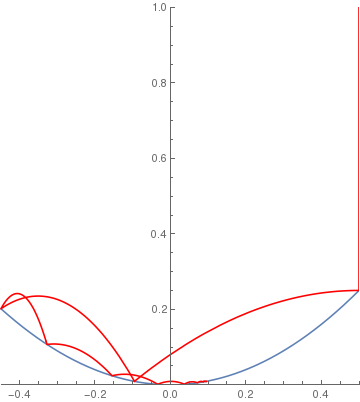
squareramp[x_] := If[x < 4, x^2, 0]; BouncingBall[.7, squareramp, {.5, 1}] |
 |
|
(*Cubic ramp*)
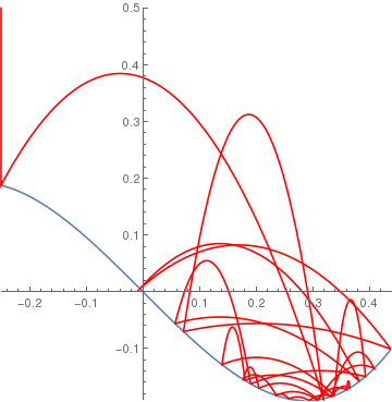
cuberamp[x_] := If[-1 < x < 5, 4 (x^3) - x, 0]; BouncingBall[.9, cuberamp, {-0.25, .5}] |
 |
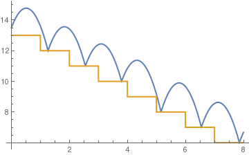
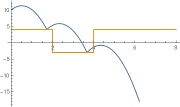
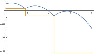
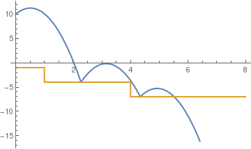
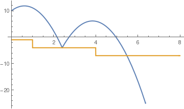
Example 4: Now we consider a bouncing ball on stairs.
c = .75;
sol = NDSolve[{y''[t] == -9.8, y[0] == 13.5, y'[0] == 5, a[0] == 13, WhenEvent[y[t] - a[t] == 0, y'[t] -> -c y'[t]], WhenEvent[Mod[t, 1], a[t] -> a[t] - 1]}, {y, a}, {t, 0, 8}, DiscreteVariables -> {a}];
Plot[Evaluate[{y[t], a[t]} /. sol], {t, 0, 8}, PlotStyle -> Thick]
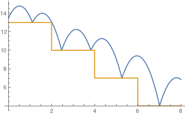
(*tall steps*)
c= .6;
sol = NDSolve[{y''[t] == -9.81, y[0] == 13.5, y'[0] == 5, a[0] == 13, WhenEvent[y[t] - a[t] == 0, y'[t] -> -c y'[t]], WhenEvent[Mod[t, 2], a[t] -> a[t] - 3]}, {y, a}, {t, 0, 8}, DiscreteVariables -> {a}];
Plot[Evaluate[{y[t], a[t]} /. sol], {t, 0, 8}, PlotStyle -> Thick]
(*positive to negative steps*)
c = .5;
sol = NDSolve[{y''[t] == -9.81, y[0] == 10, y'[0] == 5, a[0] == 4, WhenEvent[y[t] == a[t], y'[t] -> -c y'[t]], WhenEvent[Mod[t, 2], a[t] -> 1 - a[t]], WhenEvent[ y[t] < a[t] , y''[t] = -y'[t]]}, {y, a}, {t, 0, 4}, DiscreteVariables -> {a}];
Plot[Evaluate[{y[t], a[t]} /. sol], {t, 0, 8}, PlotStyle -> {Thick, Thick}]
 |
 |
 |
| standard stairs | tall steps | positive to negative steps |
c= .7;
sol = NDSolve[{y''[t] == -9.81, y[0] == 10, y'[0] == 5, a[0] == 3, WhenEvent[y[t] == a[t], y'[t] -> -c y'[t]], WhenEvent[a[t] == y[t], a[t] -> 1 - (a[t])^2], WhenEvent[ y[t] < a[t] , y''[t] = -y'[t]]}, {y, a}, {t, 0, 10}, DiscreteVariables -> {a}];
Plot[Evaluate[{y[t], a[t]} /. sol], {t, 0, 8}, PlotStyle -> {Thick, Thick}]
(*time based steps*)
c = .5;
sol = NDSolve[{y''[t] == -9.81, y[0] == 10, y'[0] == 5, a[0] == -1, WhenEvent[y[t] == a[t], y'[t] -> -c y'[t]], WhenEvent[t == -a[t], a[t] -> a[t] - 3], WhenEvent[ y[t] < a[t] , y''[t] = -y'[t]]}, {y, a}, {t, 0, 5}, DiscreteVariables -> {a}];
Plot[Evaluate[{y[t], a[t]} /. sol], {t, 0, 8}, PlotStyle -> {Thick, Thick}]
c = 0.8;
sol = NDSolve[{y''[t] == -9.81, y[0] == 10, y'[0] == 6, a[0] == -1, WhenEvent[y[t] == a[t], y'[t] -> -c y'[t]], WhenEvent[t == -a[t], a[t] -> a[t] - 3], WhenEvent[ y[t] < a[t] , y''[t] = -y'[t]]}, {y, a}, {t, 0, 5}, DiscreteVariables -> {a}];
Plot[Evaluate[{y[t], a[t]} /. sol], {t, 0, 8}, PlotStyle -> {Thick, Thick}]
 |
 |
 |
| corner to corner bounces | time based steps | elastic bounce |
Controllability of Linear Systems
The concept of controllability analysis plays a crucial role in many regulation problems, such as the stabilization of unstable systems using feedback, tracking problems, obtaining optimal control strategies, or, simply prescribing an input that has a desired effect on the state. It considers whether a system can be steered from an arbitrary initial state to any desired final state using appropriate control inputs within a given time frame. Controllability in linear systems is governed by the qualities of the system’s state matrix and control matrix. A system is considered controllable if the reachable states can span its state space under the effect of control inputs. This feature is critical in engineering and control theory because it underpins the design and execution of successful control techniques for a wide range of applications, including robotics and aerospace, as well as economics and chemical processes.
- The operator C is onto (surjective).
- The operator C✶ is onto.
- The Gramian matrix \[ \mathbf{W}\left( t_0 , t_1 \right) = C\,C^{\ast} = \int_{t_0}^{t_1} \, e^{\mathbf{A}\left( t_1 - \tau \right)} \,\mathbf{B}\,\mathbf{B}^{\mathrm T} \,e^{\mathbf{A}^{\mathrm T} \left( t_1 - \tau \right)} \,{\text d}\tau \] is non-singular.
Example 5: ■
Example 6: ■
- PBH Rank Condition: . Rank[s Iₙ − A, B] = n, ∀ s ∈ ℂ.
- PBH Eigenvector Condition: the relationship v A = λv implies v B ≠ 0, where v is a left eigenvector of A associated with the eigenvalue . λ.
Example 7: the satellite system
page 280 at in A Course in Linear Algebra by George & ■
Return to Mathematica page
Return to the main page (APMA0340)
Return to the Part 1 Matrix Algebra
Return to the Part 2 Linear Systems of Ordinary Differential Equations
Return to the Part 3 Non-linear Systems of Ordinary Differential Equations
Return to the Part 4 Numerical Methods
Return to the Part 5 Fourier Series
Return to the Part 6 Partial Differential Equations