In this section, we consider vectors as n-tuples and some of their
configurations when all entries are numbers from a field of either ℤ, all integers, or ℚ, rational numbers, or ℝ, real numbers, or ℂ, complex numbers. It is convenient to use Dirac's formalism for implementing duality in considering numeric vector x = (x₁, x₂, … , xn) ∈ 𝔽n (which is a Cartesian product of n copies of field 𝔽) as either ket-vector ∣x⟩ (or simply vector) or bra-vector ⟨x∣ (also is known as a covector), independently of the form in which vector x is presented.
form a standard basis in 𝔽n, independently which of four fields (ℤ or ℚ or ℝ or ℂ) is in use. We also use the same notation {e₁, e₂, … , en} for standard basis vectors written as row vectors or column vectors.
Any vector space (𝔽n in particular) admits infinitely many bases (see Part 3 for detail). However, when we deal with 𝔽n, every vector is assumed to be stuck with the standard basis upon using it as an n-tuple: x = (x₁, x₂, … , xn).
In applications, vectors usually have some physical meanings, but humans with computers would like to present vectors in mathematical forms suitable to the theoretical model under consideration. So we consider, besides n-tuples, vector representations in two forms: as column vectors and as row vectors (in part 5 you will see another vector appearance as diagonals in a square matrix).
Now we treat n-tuples (or lists of size n) as column vectors:
where we denote by 𝔽n×1 = 𝔽n,1 the vector space of n-column vectors with entries from field 𝔽 (either ℤ or ℚ or ℝ or ℂ). This column space is matrix space, its dimensions contain two numbers (separated either by comma or by × sign, which in this context is not the multiplication sign. Here it stands for the English word "by" so that "nx1" is understood to mean "n by 1", "n" for number of rows and "1" for number of columns). Since entries of n-tuple are exactly the same as entries in column vector, with the same order, it is just another form of viewing the same vector. In order to address this situation, mathematicians call these two spaces 𝔽n and 𝔽n×1isomorphic and their relationship is denoted as 𝔽n ≌ 𝔽n×1. I hope that it is clear that if 𝔽n is isomorphic to 𝔽n×1, then 𝔽n×1 is also isomorphic to 𝔽n because you can uniquely identify the n-tuples from its column counterpart. Notation 𝔽n,1 for space of column vectors is also widely used.
We can also transfer 𝔽n into vector space of row vectors:
where 𝔽1×n = 𝔽1,n is the vector space of row vectors of size n. While a vector written as an n-tuple and as a row vector look identical to human eyes, a computer solver treats these two objects differently: row vectors and column vectors have two dimensions inherited from their matrix representations. On the other hand, an n-tuple is just a one dimensional array and has a single dimension, its size.
Of course, 𝔽n×1 and 𝔽1×n, are isomorphic to the direct product, 𝔽n ≌ 𝔽n×1 = 𝔽n,1 ≌ 𝔽1×n = 𝔽1,n, but these vector spaces have slightly different structures. Your software package distinguishes an n-tuple (or list of size n) from a column vector or a row vector that have dimensions n×1 and 1×n, respectively. The following example demonstrates how Mathematica treats different kinds of numerical vectors.
Example 1:
We start with a simple 3-tuple:
v = {1, 2, 3}
{1, 2, 3}
Dimensions[v]
{3}
In order to display this vector, we use two commands:
Although Mathematica presents an n-tuple (as an element of 𝔽n) in the column form exactly as the pure column vector, it treats this vector differently from column vector:
SameQ[v, v2]
False
Here is a summary of the output above in table form
As this example shows, Mathematica treats differently vectors written in different forms: n-tuples (as elements of 𝔽n) that are identified in curly brackets { … } while row vectors and column vectors are defined as matrices {{ … }} and {{…}, {…}, … , {…}}, respectively.
Example 2:
The code presented in Example 1 shows that Mathematica distinguishes a 3-tuple from a column vector, and assigns different dimensions to these vectors.
We can convert an n-tuple into a row vector as
rowVector = ArrayReshape[v, {1, Length[v]}]
{{1, 2, 3}}
Dimensions[%]
{1, 3}
rowVector1 = {v}
{{1, 2, 3}}
Converting a list into column vector can be accomplished as follows:
Note that Dimensions of colVector are reverse of rowVector
Dimensions[colVector]
{3, 1}
colVecto1r = List /@ v
{{1}, {2}, {3}}
As it is seen from Mathematica's codes, this computer algebra system distinguishes lists from column vectors and row vectors. Recall that we denote by 𝔽1,n = 𝔽1×n the vector space of row vectors with entries from field 𝔽. Note that the dimensions of this space are inherited from matrix space, therefore, there are two forms of writing its dimensions either with comma or with product sign.
■
End of Example 2
Matrices as Operators
Now we come to the main issue of linear transformations: how to define in a practical way a linear map between two vector spaces 𝔽n and 𝔽m. To achieve this, we need to transfer the direct product form of 𝔽n into matrix form (for any positive integer n ∈ ℕ+ = {1, 2, 3, …}). In other words, we need to resettle n-tuples into matrix forms, either as column vectors or as row vectors. This will allow us to multiply matrices with vectors written in matrix forms.
Once direct product 𝔽n is transferred into either 𝔽n×1 (called column vector space) or 𝔽1×n (known as a row vector space), we can apply matrix multiplications to elements from these vector spaces. In particular, if A is an m × n matrix with entries from field 𝔽, we can multiply it from left on column vector (which is n×1 matrix) to obtain an m×1 matrix, which is again a column vector of size m.
The graphic above shows that composition of matrix/vector operation (left matrix multiplication shown in the last line) with isomorphism mappings 𝔽n ≌ 𝔽n×1 and 𝔽m×1 ≌ 𝔽m defines the linear transformation LA from 𝔽n into 𝔽m.
The mathematical operator, ≌, is a special form of equal sign that means "All Equal To"
Similarly, we can define a dual linear transformation RA from 𝔽m into 𝔽n using vector/matrix operation (multiplication by a matrix from right shown in the last line), as the following graphic shows
The reader is urged to make a close comparison of the preceding two graphics, taking particular note of the difference between them specifically in superscript notation and direction of arrows. Recognize the importance of two shorthand symbols: the statement LA: at the beginning of the first line of the first graphic means "Linear Transformation of Matrix A from the Left" and :RA at the end of the first line of the second graphic means "Linear Transformation of transformed Matrix A from the Right back to the original Matrix A."
Any numerical vector r = (r₁, r₂, … , rn) ∈ 𝔽n can be considered as a ket-vector ∣r⟩ (which is usually identified with a column vector) or as a bra-vector ⟨r∣ (which is usually written as a row vector). These representations as column and row vectors were made in the first part of twentieth century (when computers were not available). The main idea of this portrayal is to help people identify action of bra-vector on ket-vector via matrix multiplication (row times column). Duality of such delineation becomes crystal clear: bra-vector ⟨r∣ acts on ket-vector ∣x⟩ = (x₁, x₂, … , xn) and ket-vector can also act on bra-vector resulting in a numerical value:
The linear combination of numerical values in the right-hand side of the latter is known as the dot product of two equal-length vectors (independently on whether they are n-tuples or columns or rows):
However, bra-ket notation ⟨r∣x⟩ and dot product r • x are conceptually different in a subtle way despite that they both are expressed via the same formula. The Dot product is defined for two vectors from the same vector space. In practical applications, these vectors have the same units. The bra-ket notation is used to represent the duality of acting one vector on another vector; note that bra-vectors and ket-vectors often have different units.
For example, you visit a store and check a price list, which can be considered as a bra-vector ⟨r∣ with units $/kg. When you buy some products, say you choose several apples and some kiwis; upon their weighing, you were given ket-vector, which consists of the weights of your products, ∣x⟩. What a cashier does is just apply the price list (bra vector) to weights of your chosen fruits (ket vector), providing you a total bill, a number in dollars that you have to pay. So you can represent the cashier as ⟨r∣x⟩ that assigns a number to ket vector and bra vector. In economics, this number is called a "total." In physics, this number is called an "observation."
There is another, algebraic, way of describing how the bra- and ket-vectors interact. Continuing with our fruit example, let us assume that apples cost $1 per kg and you want four kg of apples. The equation for finding the price is
Notice initially the equation has incompatible units when we try to divide kilograms into dollars. Now, as described above, the cashiering function serves to eliminate one unit, kg, cleanly by cancelation, leaving us with the correct number AND the single, correct unit, in this case, dollars. The dot product accomplishes this as it is unit-free. The bra- and ket- convention permits units because bra- and ket- vectors represent physical measures (speed, heat, etc.) where units need to be preserved. This is less true in economics as the final result in dollars is often assumed from the context.
Be aware that representation of a bra vector as a row vector and a ket-vector as a column vector may lead to the wrong conclusion that action of bra on ket (and vice versa) can be represented by vector product (same as "dot product"):
which is not a number but 1 × 1 matrix. Of course, this matrix is equivalent to the number, but it is still the matrix, from which you need to extract the entry. Situation is similar with your bank account: you have money in a bank, but to see cash, you need to visit a bank branch or ATM and withdraw the money.
It is a customary to say that a linear functional (or bra-vector or covector) acts on or
operates a ket vector, which results in numerical output. In physics, the result of operation on a ket-vector is known as an observation.
This applies equally to economics in the grocery example. Suppose you buy apples, bananas, plums and oranges. The bra-vector of prices is, in dollars per kg:
braVec = {1.1, .75, 1.25, .95}(* dollars per kg *);
The ket-vector of weights is:
ketVec = {1.2, .6, 2, 3}(* kilograms *);
The amount you owe the cashier is (note that units in dollars is assumed from the context)
braVec . ketVec
7.12
Were you to enter this information into a spreadsheet, similar to what the cashier's machine is doing, you would have subtotals at the end of each additional line entry. It might look like this
Example 3:
In case of real three-dimensional vector space ℝ³, it is possible to give a geometric interpretation of a linear equation and show that its solution set is uniquely defined by a perpendicular vector.
Let us consider a 3-vector r = (2, 1, −1) ∈ ℝ³.
Treating this 3-vector as a covector, we operate with it on arbitrary ket-vector ∣x⟩ = (x₁, x₂, x₃):
\[
\langle \mathbf{r} \mid \mathbf{x} \rangle = \left( 2, 1, -1 \right) \bullet \left( x_1, x_2 , x_3 \right) = 2\,x_1 + x_2 - x_3 .
\tag{3.1}
\]
When entering this information into a notebook, it is convenient to get rid of subindexing. Therefore, we use x1, x2, x3 instead of x₁, x₂, x₃. Substituting accordingly into our solution to the linear equation we just obtained, we get
We know that t = x1 and s = x2 so the final matrix in (3.2) above is
MatrixForm[{t, s, x3New}]
\( \displaystyle \quad \begin{pmatrix}
t \\ s \\ s + 2\,t
\end{pmatrix} \)
r = {2, 1, -1};
x = {x1, x2, x3};
r . x
2 x1 + x2 - x3
First, we check what 3-vectors are mapped by r into zero; so we need to solve the linear equation:
\[
2\,x_1 + x_2 - x_3 = 0 \qquad \Longrightarrow \qquad x_3 = 2\,x_1 + x_2 .
\]
Reduce[r . x == 0, x]
x3 == 2 x1 + x2
Therefore, ket-vectors that are orthogonal to r (in the sense that their dot product with the bra-vector vanishes, ⟨r∣ • ∣x⟩ = 0) constitute a two-dimensional vector space
\[
\mathbf{r}^{\perp} = \left\{ \begin{bmatrix} x_1 \\ x_2 \\ x_3 \end{bmatrix} \in \mathbb{R}^{3\times 1} \, : \ x_3 = 2\,x_1 + x_2 \right\} = \left\{ \begin{bmatrix} x_1 \\ x_2 \\ 2\,x_1 + x_2 \end{bmatrix} \, : \ x_1, x_2 \in \mathbb{R} \right\} .
\]
So the annihilator of r is a two-dimensional hyperspace in ℝ³ that is orthogonal to the bra-vector ⟨r∣:
\[
\mathbf{r}^{\perp} = \left\{ t \begin{bmatrix} 1 \\ 0 \\ 2 \end{bmatrix} + s \begin{bmatrix} 0 \\ 1 \\ 1 \end{bmatrix} = \begin{bmatrix} t \\ s \\ 2\,t + s \end{bmatrix} \, : \ t,s \in \mathbb{R} \right\} ,
\tag{3.2}
\]
where arbitrary real numbers t and s are used instead of x₁ and x₂. This hyperspace r⊥ is spanned on two vectors u₁ = (1, 0, 2) and u₂ = (0, 1, 1). These vectors are not orthogonal because
\[
\mathbf{u}_1 \bullet \mathbf{u}_2 = \left( 1, 0, 2 \right) \bullet \left( 0, 1, 1 \right) = 2 \ne 0.
\]
It is convenient to choose two orthogonal vectors that span hyperplane r⊥, so we use the cross product operation because it automatically provides orthogonality:
Mathematica provides us two orthogonal vectors
\[
\mathbf{v}_1 = \left( 1, -2, 0 \right) \qquad \mbox{and} \qquad \mathbf{v}_2 = \left( -2, -1, -5 \right) ,
\]
with property
\[
\mathbf{v}_1 \bullet \mathbf{v}_2 = \left( 1, -2, 0 \right) \bullet \left( -2, -1, -5 \right) = 0.
\]
We check with Mathematica that these two vectors are elements of r⊥:
v1 = {1, 2, 0}; v2 = {-2, -1, -5};
v1 . r
v2 . r
0
0
Instead of using brute force method for determination of vectors v1 = r × (0, 0, 1) and v2 = r × v1, we can utilize our knowledge of vectors u1 or u2 that are orthogonal to r.
r = {2, 1, -1};
Cross[r, {1, 0, 2}]
{2, -5, -1}
with
r . {2, -5, -1}
0
or
Cross[r, {0, 1, 1}]
{2, -2, 2}
with
r . {2, -2, 2}
0
Therefore, we can use also the following two pairs of orthogonal vectors
\[
\begin{pmatrix} 1&0&2 \\ 2&-5&-1 \end{pmatrix} \qquad \mbox{or} \qquad \begin{pmatrix} 0&1&1 \\ 2&-2&2 \end{pmatrix} .
\]
Next, we solve the inhomogeneous problem
Solve[r . x == b, x3][[1, 1]]
x3 -> -b + 2 x1 + x2
Note that this last result is the same as our prior value for x3 when b = 0.
(Solve[r . x == b, x3] /. b -> 0)[[1, 1]]
x3 -> 2 x1 + x2
\[
\langle \mathbf{r} \mid \mathbf{x} \rangle = \left( 2, 1, -1 \right) \bullet \left( x_1, x_2 , x_3 \right) = 2\,x_1 + x_2 - x_3 = b ,
\tag{3.3}
\]
where b is an arbitrary real number. Solving equation (3.3), we get
\[
x_3 = -b + 2\,x_1 + x_2 ,
\]
which leads to two dimensional hyperplane (it is not a linear space)
\[
S_b = \begin{bmatrix} 0 \\ 0 \\ -b \end{bmatrix} + \mathbf{r}^{\perp} = \left\{ \begin{bmatrix} t \\ s \\ -b + 2\, t + s \end{bmatrix} \, : \ t, s \in \mathbb{R} \right\} .
\]
There is an infinite number of planes orthogonal to r. Values for b other than 0 produce planes at different points along r. For instance, if b = 1, functional ⟨r∣ maps vectors into 1; hence,
\[
2\,x_1 + x_2 - x_3 = 1 \qquad \Longrightarrow \qquad x_3 = -1 + 2\,x_1 + x_2 .
\]
Reduce[r . x == 1, x]
x3 == -1 + 2 x1 + x2
This equation shows that the bra-vector ⟨r∣ acts on these vectors giving output 1 when ket-vectors belong to the plane S₁ parallel to the hyperspace ⟨r∣⊥.
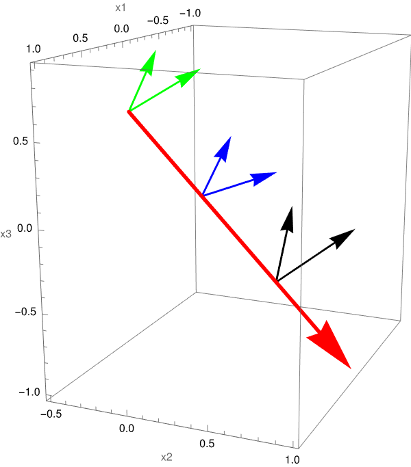
Now we plot two generating vectors for ⟨r∣⊥ and Sb for two numerical values of b.
Here are three pairs of vectors attached along vector r at various points.
Figure 1: Action of bra-vector ⟨(2, 1, −1)∣.
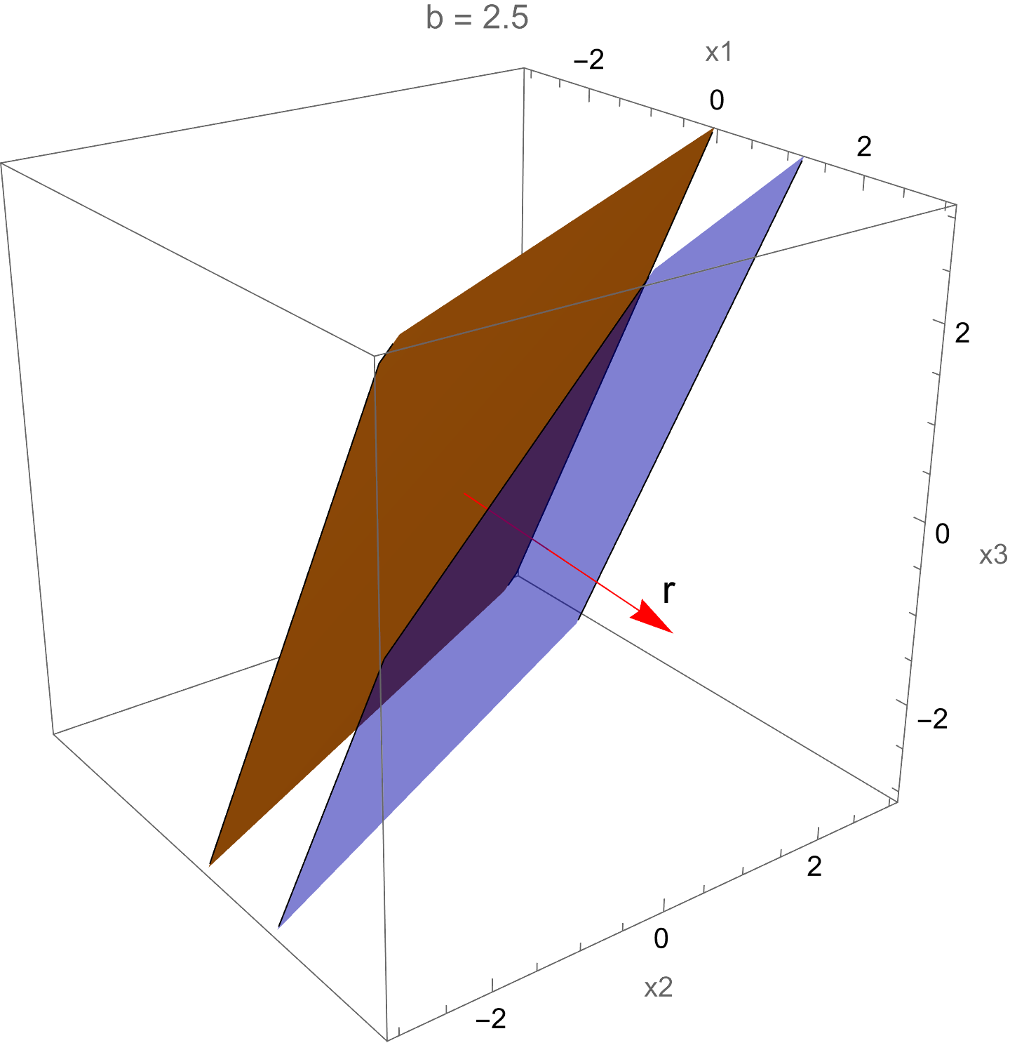
Below we see how increasing b from 0 to 4 changes the position of the plane that is, at all times, orthogonal to vector r:
However, this m × n matrix A cannot operate on row vectors from left because their dimensions do not match. Nevertheless,, it can operate on row vector from right! if we have an m row vector (which is 1×m matrix) y, we can represent the matrix as an m row vector with n columns as entries:
Therefore, every m × n matrix A ∈ 𝔽m,n can operate from left on n-column vectors to produce m-column vectors, or it can operate from right on m row vectors to produce output of n row vectors.
Theorem 1:
If A is an m × n matrix with entries from field 𝔽 (which is either ℤ or ℚ or ℝ or ℂ), then the transformation 𝔽n×1 ∋ x ↦ A x ∈ 𝔽m×1 is linear.
Similarly, multiplication from right, defines the linear transformation: 𝔽1×m ∋ y ↦ y A ∈𝔽1×n.
Example 4:
For instance, multiplication of 2 × 4 matrix A and 4 × 1 matrix v (which is a 4-column vector) yields
A={{2,-3,1,2},{5,1,2,4}};
v ={1,-1,2,-3};
colVector = List /@ v
A.colVector
{{1}, {-4}}
Every m × n matrix A can be written as an m × 1 matrix (which is a column vectors of size m) with row vectors of size n as entries. In our example, we have
Then multiplication from left of column vector v by matrix A produces another column vectors, but of size m. In this case, we say that matrix Aoperates on v and transfer it into another vector u = A v. Its action on column vector can be written using dot product:
For historical reasons, it is a custom to write functions at the left of argument. Most likely this form of writing is inherited from European languages---all of them write from left to right. That is way we write sin(x) but not (x)sin. Also all computer solvers utilize the same approach by writing a function at the left of its argument.
In what follows, we will always consider operation of matrix A on column vectors from left. Then equation \eqref{EqTransform.2} defines a linear transformation from 𝔽n,1 ≌ 𝔽n into 𝔽m,1 ≌ 𝔽m.
For any two positive integers m and n, a matrix A ∈ 𝔽m,n defines a linear transformation TA : 𝔽n ⇾ 𝔽m by
\[
\mathbb{F}^n \ni {\bf x} \cong \{ {\bf x}\} \in \mathbb{F}^{n,1} \ \mapsto \left\{ {\bf A\,}\{ {\bf x}\} \right\} \in \mathbb{F}^{m,1} . %\cong {\bf A\,x} \in \mathbb{F}^m .
\]
Since matrix multiplication (either from lef or from tight) is a linear transformation, it is often called an operator that transfer vectors from 𝔽n×1 into 𝔽m×1.
So the multiplication from left of a vector by a matrix “transforms” the input vector into an output column vector, possibly of a different size.
More over this transformation happens in a “linear” fashion.
Any x whose image under T is b must satisfy equation (4.2). From (4.3), it is clear that equation (5.2) has a unique solution. So there is exactly one x whose image is b.
The vector c is the range of T if c is the image of some x. This is just another way of asking if the system A x = c is consistent. To find the answer, row reduce the augmented matrix:
\[
\left[ \begin{array}{cc|c} \phantom{-}1 & -2 & 1 \\ \phantom{-}3 & \phantom{-}4 & 3 \\ -5 & \phantom{-}1 & 2 \end{array} \right] \, \sim \, \left[ \begin{array}{cc|c} 1 & -2 & 1 \\ 0 & 10 & 0 \\ 0 & -9 & 7 \end{array} \right] \, \sim \, \left[ \begin{array}{cc|c} 1 & 0 & 1 \\ 0 & 1 & 0 \\ 0 & 0 & 7 \end{array} \right] .
\]
The third equation, 0 = 7, shows that the system A x = c is inconsistent. Hence, c is not in the range of T.
■
End of Example 5
The question in Example 5(d) is a uniqueness problem for a system of linear equations translated into the language of matrix transformations: is b the image of a unique x in ℝn? Similarly, Example 4(e) is an existence problem: does there exist an x whose image is c = A x?
Example 6:
Recall from the section on Vectors that the set of
all ordered n-tuples or real numbers is denoted by the symbol ℝn, for any positive integer n ∈ ℕ+ = {1, 2, 3, … }. It is customary
to interpret ordered n-tuples in matrix notation as column vectors. For example, the matrix
can be used as an alternative to \( {\bf v} = \left[ v_1 , v_2 , \ldots , v_n \right] \quad\mbox{or}\quad
{\bf v} = \left( v_1 , v_2 , \ldots , v_n \right) . \) The latter is called the comma-delimited form of a
vector and former is called the row-vector form.
In ℝn, the vectors e1 = (1, 0, 0, … , 0), e2 = (0, 1, 0, … , 0), … , en = (0, 0, … , 0, 1)
form an ordered basis for n-dimensional real space, and it is called the standard basis. Its dimension is n because there n linearly independent vectors e1, e2, … , en that generate ℝn.
For example, the vectors
Although the latter represents a linear system of equations, we could view it instead as a transformation T that maps a
vector x from 𝔽n into the vector T(x) from 𝔽m generated by multiplying the corresponding column vector x ∈ 𝔽n×1 on the left by A.
We call T a matrix transformation and denote by TA : 𝔽n ⇾ 𝔽m (it is also frequently denoted by LA to emphasize that matrix A acts from left). This transformation (either TA or LA) is also called matrix operator, especially when m=n. This transformation is generated by
matrix multiplication from left:
Theorem 2:
For every m × n matrix A. the matrix transformation
\( T_{\bf A}:\, \mathbb{R}^n \to \mathbb{R}^m \) has the following properties for all vectors
v and u and for every scalar k:
so multiplication by zero maps every vector from \( \mathbb{R}^m \) into the zero vector
in \( \mathbb{R}^n . \) Such transformation is called the zero transformation from
\( \mathbb{R}^m \) to \( \mathbb{R}^n . \)