The Dual of a Dual Space

Example 11: The "dual" of a vector is the linear transformation that it encodes onto the real or complex number. Another way of expressing the same concept is: the "dual" of a linear transformation from space to one dimension (ℂ or ℝ) is a certain vector in that space. A non-mathematician might, as a result of this, ascribe somewhat magical properties to the dot product because that is just what the dot product does: locate an answer to a vector question on the real number line or complex plane. Mathematicians and physicists have long studied the notion of Duality and have given various interpretations of it. One of these is that when two different mathematical abstractions share [some] properties, they are endowed with a correspondence that is very useful in practice. More complex transformations, such as Fourier, permit one to make theoretical progress on otherwise intractable problems in the transform space, achieving a result otherwise not possible and then transform that result back to the original for a practical answer that was out of reach in the pre-transformed expression.

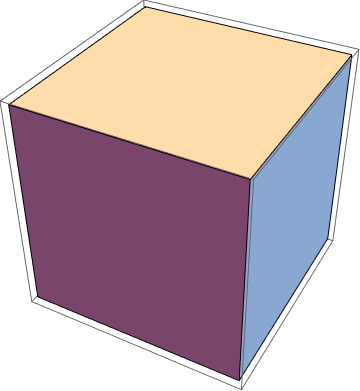
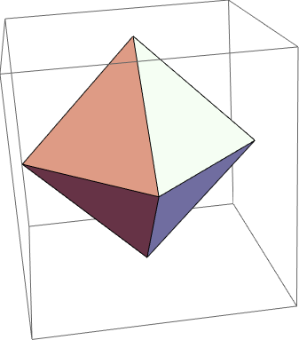
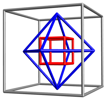
The figure below is a simple example of duality and how one may move easily from one to the other and back. Notice the commonality of six and eight in each figure. Each object has a set of 6 somethings and a set of eight somethings, but they are not the same things. For the cube it is six faces and eight vertices. Count the equivalent for the octahedron. Note the each have the same number of edges. There is a mathematical relation between the cube and the octahedron which permits one to "convert" one shape to the other; reversing that process returns to the original shape. Naturally, there is a scale factor involved, explaining why the outside cube is much larger than the one inside. The mathematical relationship is described above where the center of the faces of one are linked, thereby creating the other.

The preceding geometric duality construction can be made for all Platonic solids. Here is a list of these regular polyhedra.

	Vertices (v)	Edges (e)	Faces (f)	f - e + v
tetrahedron	4	6	4	2
cube	8	12	6	2
octahedron	6	12	8	2
dodecahedron	20	30	12	2
icosahedron	12	30	20	2

The exchange of the numbers of faces (f) and vertices (v)

(leaving the number e of edges invariant) produces a symmetry ■

Example 12: A typical linear programming problem that was first formulated by the Russian scientist Leonid Kantorovich in 1939, asks to minimize the cost function c • x subject to constraints: where A is an m × n matrix with real coefficients and b ∈ ℝ^m×1 ≌ ℝ^m. As usual, the cost function c • x = c₁x₁ + ⋯ + c_nx_n is a dot product of two vectors. Any vector satisfying the constraint conditions is called feasible.

There are known two well-known methods to solve this optimization problem: the simplex _algorithm (invented by George Dantzig during the second world war) and Karmarkar’s Method (1984).

The dual problem starts from the same A, b, and c, and reverses everything. In the primary problem, c is in the cost function and b is in the constraint, In the dual, b and c are switched, The dual unknown y ∈ 𝔽^{1, m} is a row vector with m components, and the feasible set has y A ≤ c instead of A x ≥ b. In short, the dual of a minimum problem is a maximum problem. Now y ≥ 0: The dual of this problem is the original minimum problem. A set of all solutions y ∈ ℝ^1×m ≌ ℝ^m satisfying (12.2) is called a polyhedron. There is a symmetry between the primal and dual problems. The simplex method applies equally well to a maximization—anyway, both problems get solved at once.

If optimal vectors do not exist, there are two possibilities: Either both feasible sets are empty, or one is empty and the other problem is unbounded (the maximum is +∞ or the minimum is −∞).

The central question of economics is how to allocate scarce resources amongst alternative ends. This turns into a series of sub-issues:

1. How much of what to apply and when?
2. How does the application of any particular factor/resource change the output in both absolute and relative terms?
3. What is the best combination of resources that produces the most efficient result?

The analytical technology required to answer these questions involves a process known as "Optimization" which, in practical terms, becomes finding the maximum or a minium of a function. This can require intertwined functions. For instance, the optimization of net income (revenue minus cost) involves the simultaneous maximization of revenue and minimization of cost.

Life involves trade-offs. Constraints force trade-offs into the picture. You can't go to the movie and the ballgame on the same night. One must make choices. A rational life means making choices which optimize your time/happiness/profits/career/retirement savings. The ideas of maximization and minimization become more interesting in the presence of constraints. Mathematica has very highly evolved algorithms for solving these kinds of problems.

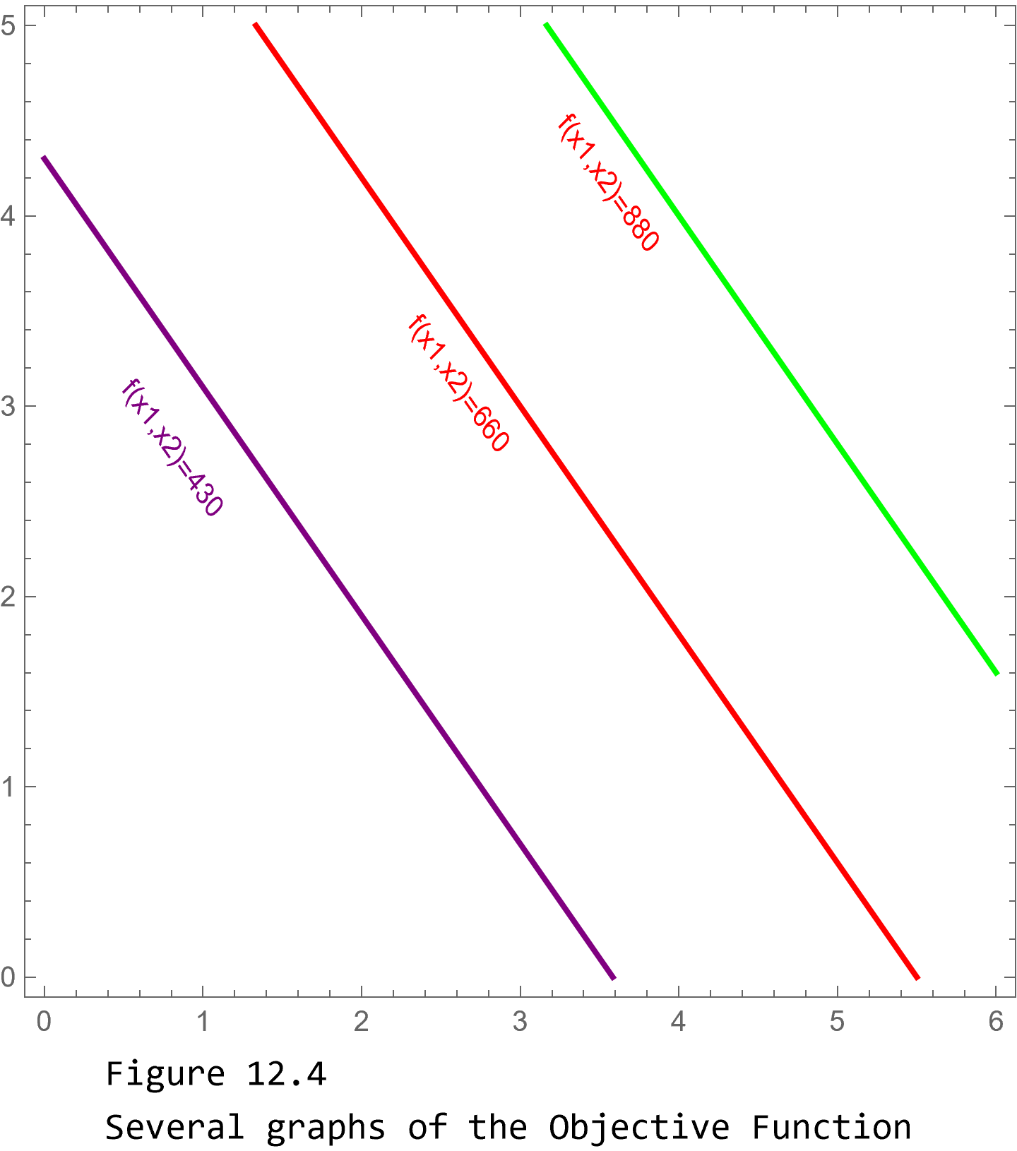
It all begins with stating the goal as an "objective function." This is the mathematical expression of what you wish to achieve. So here we have some x and y (inputs, products, choices) that must be combined in a certain way to get us where we want to be.

In order to illustrate the concepts, we consider a simple primal minimization problem:

minimize a cost function \( \displaystyle \qquad f(x_1 , x_2 ) = 120\,x_1 + 100\, x_2 \qquad \iff \qquad f({\bf x}) = {\bf c} \bullet {\bf x} , \quad \) where c = (120, 100) and x = (x₁, x₂),

subject to constraints:

It is convenient to rewrite these constraints in vector form:

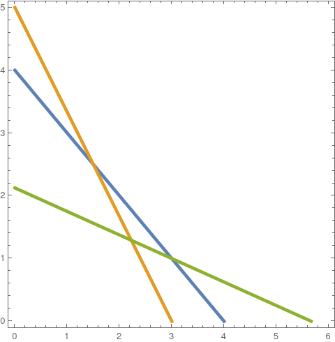
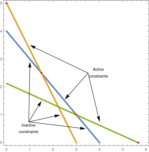
First, we find the solution of the formulated primal minimization problem geometrically, and then solve it analytically. So we plot the constraint functions

cntrPlt1 = ContourPlot[{2 x + 2 y == 8, 5 x + 3 y == 15, 3*x + 8*y == 17}, {x, 0, 6}, {y, 0, 5}, ContourStyle -> Thickness[0.01]]; LLabeled[%, "Figure 12.1: Constraint Lines"]abeled[%, "Figure 12.1: Constraint Lines"]

Then we cut off parts of these lines that do not define the feasible region.

pt1 = Solve[{2 x1 + 2 x2 == 8, 5 x1 + 3 x2 == 15}, {x1, x2}][[1, All, 2]]; pt2 = Solve[{2 x1 + 2 x2 == 8, 3 x1 + 8 x2 == 17}, {x1, x2}][[1, All, 2]]; pt3 = {Solve[3 x1 + 8 x2 == 17 /. x2 -> 0, x1][[1, 1, 2]], 0}; pt4 = {0, 5}; pt5 = {5, .25}; pts1 = Show[ Graphics[{Red, PointSize -> Medium, Point[#]}] & /@ {pt1, pt2, pt3, pt4}]; arr1 = Graphics[{Arrow[{{3.5, 2.5}, {1, 3.5}}], Arrow[{{3.5, 2.5}, {2.5, 1.55}}], Arrow[{{3.5, 2.5}, {4, .75}}], , Arrow[{{.95, .75}, {1.5, 1.5}}], Arrow[{{.95, .75}, {1, 2.9}}], Arrow[{{.95, .75}, {2.3, 1}}], Arrow[{{.95, .75}, {3.4, .5}}], Text["Inactive\nconstraints", {.95, .5}], Text["Active\nconstraints", {3.95, 2.5}]}]; sh1 = Labeled[Show[cntrPlt1, pts1, arr1], "Figure 12.2: Active Constraint Lines"]

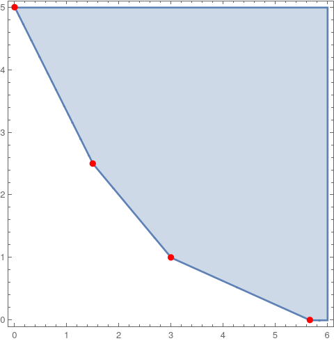
This allows us to plot the feasible region that displays the area bounded by all of the constraints. Also shown are four red points that represent so-called "corner solutions" where optimal values may be found. Note below that we have added two more constraints. Both x₁ and x₂ must be non-negative. This example is considered "stylized" in that is simplifies a context for teaching purposes.

regPlt1 = RegionPlot[{2 x1 + 2 x2 >= 8 && 5 x1 + 3 x2 >= 15 && 3*x1 + 8*x2 >= 17 && x1 >= 0 && x2 >= 0}, {x1, 0, 6}, {x2, 0, 5}]; Labeled[Show[%, pts1], "Figure 12.3: Feasible Region"]

The Simplex Method (Danzig, 1946) finds the optimal solution, which must be at one of the corners of the feasible region. Three corners of the feasible region are shown below as red points. Sections of the lines that go through two points are known as "active constraints" as they are boundaries of the feasible region. Portions of the lines which are not boundaries of the feasible region are considered "inactive constraints" as values outside the feasible region cannot result in an optimal solution.

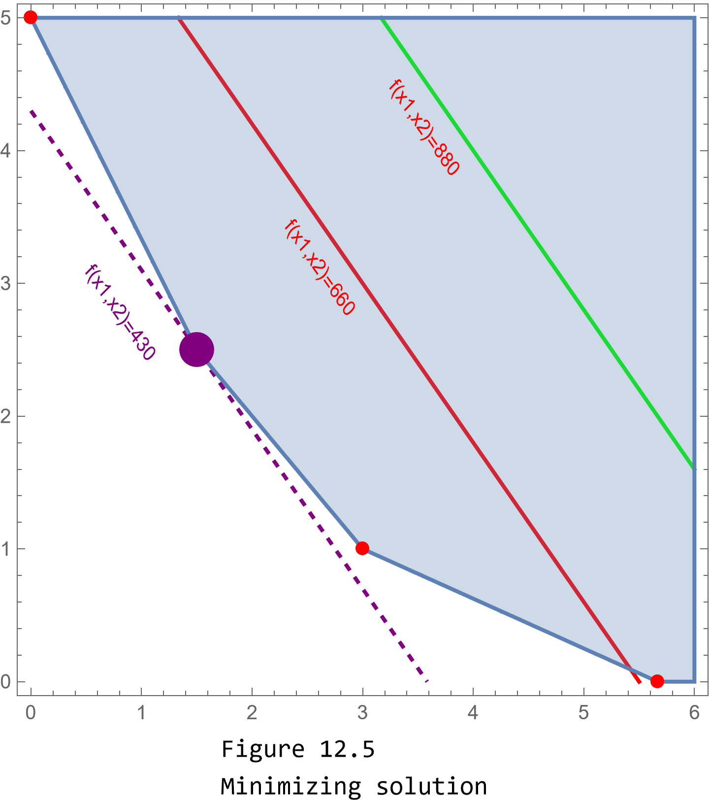
Mathematica has several ways to find the minimum of this function, here are two:

and using LinearOptimization command: Therefore, we know that the minimum is attained at the point The objective function f(x₁, x₂), when equated to a constant, defines a line. Upon using several constants, we obtain several parallel lines that may be derived using several arbitrary values, then plotted. The dashed line for the optimal solution to the objective function passes through the optimal point in purple.

 

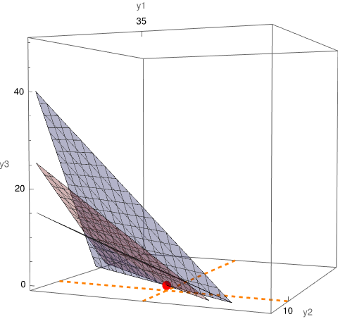
Now we formulate the dual problem: maximize the objective function       f(y₁, y₂, y₃) = 8 y₁ + 15 y₂ + 17 y₃    (note this is a function of three variables)   subject to only two constraints:

It is convenient to rewrite these constraints in vector form: We solve the dual problem with the aid of Mathematica. Hence, we know that the maximum value is attained at the same value of the objective function as we found for the primal: We also check the answer with the Gauss elimination procedure: Although Mathematica can solve this problem, here is the geometric approach. First, we plot the feasible region (polyhedron):

pt6 = Graphics3D[{Red, PointSize[.03], Point[{y1, y2, y3}]} /. soln3[[2]]]; cntrPlt3 = ContourPlot3D[{8 *y1 + 15*y2 + 17*y3 == 430, 2*y1 + 5*y2 + 3*y3 == 120, 2*y1 + 3*y2 + 8*y3 == 120}, {y1, 0, 70}, {y2, 0, 50}, {y3, 0, 50}, AxesLabel -> {"y1", "y2", "y3"}, Ticks -> {{35}, {10}, Automatic}, FaceGrids -> {{{0, 0, -1}, {{35}, {10}}}}, FaceGridsStyle -> Directive[Orange, Thick, Dashed], PlotLegends -> {"Obj Fct", "constraint-1", "constraint-2\n(because of viewpoint\nshows as only a line)"}, ViewPoint -> {1.3244723188775946`, -3.1106692576486226`, 0.13967765049131722`}, ContourStyle -> {{Red, Opacity[0.3]}, {Blue, Opacity[0.3]}, {Green, Opacity[0.3]}}]; Labeled[Show[cntrPlt3, pt6], "Figure 12.6: Optimum point (red), Objective function\nand \ Constraint planes"]

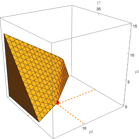
regPlt2 = RegionPlot3D[{2 y1 + 5 y2 + 3 y3 <= 120 && 2 y1 + 3 y2 + 8 y3 <= 100 && y1 >= 0 && y2 >= 0 && y3 >= 0}, {y1, 0, 70}, {y2, 0, 25}, {y3, 0, 15}, AxesLabel -> {"y1", "y2", "y3"}, Ticks -> {{35}, {10}, Automatic}, FaceGrids -> {{{0, 0, -1}, {{35}, {10}}}}, FaceGridsStyle -> Directive[Orange, Thick, Dashed], ViewPoint -> {2.4853814757635058`, -1.8372343399481694`, 1.3774791831627913`}]; Labeled[Show[regPlt2, pt6], "Figure 12.7: Optimum point (red) at edge of feasible region"]

In our example, the Primal represents the buyer who wishes to minimize his cost. He needs two inputs, x1 and x2, each with constraints imposed by others (perhaps these are different suppliers with different minimum order sizes): buy two of each and the total cost is not less than 8 (constraint g1); buy 5 x1 and 3 x2 and the total cost is not less than 15 (constraint g2); or buy 3 x1 and 8 x2 and the total cost is not less than 17 (constraint g3). Our buyer needs at least one of each (neither x1 or x2 may be zero). The resulting matrices represents information about this system. That information, together with the minimizing techniques above, tell the buyer that portions 3/2 of x1 and 5/2 of x2 is the least overall cost. When x1 costs $120 and x2 cost $100, the optimal combination at those portions equals $430: The Dual is from the prospective of the seller of x1 and x2. His goal is to maximize his revenue. His products are complements of one another. They may be acquired in any combination of two. Thus, his sales of product y are any pair selected from the set {y1, y2, y3}, permitting one of y to be zero. Shipping is accomplished through others who, in turn, impose constraints (gg1 and gg2). Using the same techniques, this time applying maximization, we determine that his optimal production combination is to produce 35 y1, 10 y2 and zero y3. At prices $8 for y1 and $15 for y2 we have the same answer, $430, for the Dual we had for the Primal:

1. Axler, Sheldon Jay (2015). Linear Algebra Done Right (3rd ed.). Springer. ISBN 978-3-319-11079-0.
2. Halmos, Paul Richard (1974) [1958]. Finite-Dimensional Vector Spaces (2nd ed.). Springer. ISBN 0-387-90093-4.
3. Katznelson, Yitzhak; Katznelson, Yonatan R. (2008). A (Terse) Introduction to Linear Algebra. American Mathematical Society. ISBN 978-0-8218-4419-9.
4. Treil, S., Linear Algebra Done Wrong.
5. Wikipedia, Dual space/