
Introduction to Linear Algebra
Systems of Linear Equations
- Introduction
- Linear systems
- Vectors
- Linear combinations
- Matrices
- Planes in ℝ³
- Equation A x = b
- Sensitivity of solutions
- Linear independence
- Plane transformations
- Space transformations
- Linear transformations
- Affine maps
- Exercises
- Answers
Matrix Algebra
- Introduction
- Manipulation of matrices
- Partitioned matrices
- Block matrices
- Matrix operators
- Determinants
- Cofactors
- Cramer's rule
- Chiò's method
- Equivalent matrices
- Elimination: A = L U
- PLU factorization
- Reflection
- Givens rotation
- Special matrices
- Exercises
- Answers
Vector Spaces
- Introduction
- Motivation
- Vector spaces
- Bases
- Dimension
- Coordinate systems
- Linear transformations
- Change of basis
- Matrix transformations
- Compositions
- Isomorphisms
- Dual transformations
- Quotient spaces
- Rank
- Solving A x = b
- Exercises
- Answers
Eigenvalues, Eigenvectors
- Introduction
- Characteristic polynomials
- Companion matrix
- Algebraic and geometric multiplicities
- Minimal polynomials
- Eigenspaces
- Where are eigenvalues?
- Eigenvalues of A B and B A
- Generalized eigenvectors
- Similarity
- Diagonalizability
- Self-adjoint operators
- Exercises
- Answers
Euclidean Spaces
- Introduction
- Euclidean space
- Bilinear transformations
- Four spaces
- Norm and distance
- Matrix norms
- Dual norms
- Dual transformations
- Examples of transformations
- Orthogonal matrices
- Self-adjoint matrices
- Unitary matrices
- Projection operators
- QR-decomposition
- Least Square Approximation
- Quadratic forms
- Exercises
- Answers
Canonical forms
- Introduction
- 2D decomposition
- 3D decomposition
- Projectors
- Direct-sum decompositions
- Cyclic decompositions
- Symmetric matrices
- Pseudoinverse
- URV-decomposition
- LU-decomposition
- QR-decomposition
- Cholesky decomposition
- Schur decomposition
- Positive matrices
- Roots
- Polar factorization
- Spectral decomposition
- CUR decomposition
- Exercises
- Answers
7. Applications
- Introduction
- Circles along curves
- TNB frames
- GPS problem
- Coriolis acceleration
- Poisson equation
- Graph theory
- Error correcting codes
- Electric circuits
- FSA
- Markov chains
- Cryptography
- Wave-length transfer matrix
- Computer graphics
- Linear Programming
- Hill's determinant
- Fibonacci matrices
- Discrete dynamic systems
- Discrete Fourier transform
- Fast Fourier transform
- Curve fitting
- Answers
8. Miscellany
- Introduction
- Circles along curves
- TNB frames
- Differential forms
- Calculus
- Vector representations
- Matrix representations
- Change of basis
- Orthonormal Diagonalization
- Generalized inverse
- Differential forms
Preliminaries
- Complex Number Operations
- Sets
- Polynomials
- Polynomials and Matrices
- Computer solves Systems of Linear Equations
- Location of Eigenvalues
- Power Method
- Iterative Method
- Similarity and Diagonalization
Glossary
Reference

This Book is licensed under Creative Commons Attribution-NonCommercial-NoDerivs 3.0 Unported License
The Wolfram Mathematica notebook which contains the code that produces all the Mathematica output in this web page may be downloaded at this link.
To enhance pedagogical effectiveness, the treatment of the dot product is presented in several distinct sections:
Curvilinear coordinates
-
Covariant (Tangent) Basis Vectors: At any point P, the natural basis vectors tangent to the coordinate curves are defined by:
\[ \mathbf{e}_i = \frac{\partial\mathbf{r}}{\partial q^i} , \qquad i = 1, 2, 3 . \]
-
The Metric Tensor (gi,j): Equipping ℝ³ with the standard Euclidean inner product ⟨ • , • ⟩, the components of the covariant metric tensor are defined as the pairwise inner products of the tangent basis vectors:
\[ g_{i,j} = \left\langle \mathbf{e}_i \mid \mathbf{e}_j \right\rangle , \qquad i,j = 1,2,3 . \]
When working in curved spaces or curvilinear coordinates, coordinate grids bend and twist. Because coordinate lines are curved, you cannot simply add two points on a curved surface together like ordinary vectors.
However, if you zoom in extremely closely on a single point P, any smooth curved surface or space looks flat. The tangent space at point P, denoted TPM (or TPℝ³ when working in 3D space), is the flat vector space formed by all possible velocity vectors of smooth curves passing through P.
- Coordinate Curves: If you hold all curvilinear coordinates constant except one (qi), the position vector r(q¹, q², q³) traces out a 1D curve in space called the qi-coordinate curve.
- Natural Basis Vectors: Taking the partial derivative\( \displaystyle \quad \mathbf{e}_i = \frac{\partial \mathbf{r}}{\partial q^i} \quad \) gives the velocity vector tangent to that specific coordinate curve at P.
- Spanning the Space: As long as the coordinate system is non-degenerate, the set of tangent vectors { e₁, e₂, e₃ } is linearly independent. Together, they form a local basis for the tangent space TPℝ³, allowing us to attach a flat Euclidean vector space (and an inner product) at every point P.
Let R be the major radius (from the center of the hole to the center of the tube) and r be the minor radius (the radius of the tube itself), with 0 < r < R. We parametrize the surface using two curvilinear coordinates (φ, θ):
-
Finding the Tangent Basis Vectors:
At any point P(θ, φ)
on the torus, the tangent space TPT²
is a 2D flat plane resting against the donut at P. Its basis is spanned by two partial derivative vectors:
-
Poloidal tangent vector (eθ): Differentiating with respect to θ
gives a vector pointing along the small cross-sectional circle of the tube:
\[ \mathbf{e}_{\theta} = \frac{\partial \mathbf{r}}{\partial\theta} = \left( -r\,\sin\theta\,\sin\phi , -r\,\sin\theta \,\sin\phi ,\ r\,\cos\theta \right) . \]
-
Toroidal tangent vector (eφ): Differentiating with respect to φ
gives a vector pointing around the main ring of the donut:
\[ \mathbf{e}_{\phi} = \frac{\partial \mathbf{r}}{\partial\phi} = \left( - \left( R + r\,\cos\theta \right) \sin\phi , \ \left( R + r\,\cos\theta \right) \cos\phi , \ 0 \right) . \]
-
Poloidal tangent vector (eθ): Differentiating with respect to θ
gives a vector pointing along the small cross-sectional circle of the tube:
-
Why This Example is Illuminating
- Position-Dependent Geometry: Every point P has its own distinct tangent plane TPT² tilted at a different angle in 3D space. A tangent vector at the top of the torus cannot be directly added to a tangent vector on the outer rim without first transporting it.
-
Varying Basis Lengths (Metric Preview): Using the standard ℝ³
dot product to measure the lengths of these basis vectors reveals:
- \( \displaystyle \quad \| \mathbf{e}_{\theta} \| = +\sqrt{\langle \mathbf{e}_{\theta} \mid \mathbf{e}_{\theta} \rangle} = r \) (constant everywhere).
- \( \displaystyle \quad \| \mathbf{e}_{\phi} \| = +\sqrt{\langle \mathbf{e}_{\phi} \mid \mathbf{e}_{\phi} \rangle} = R + r\,\cos\theta . \)
ClearAll["Global`*"]; (* 1. Define Torus Geometry and Tangent Basis Vectors *) R = 3.0; r = 1.0; pos[th_, ph_] := {(R + r Cos[th]) Cos[ph], (R + r Cos[th]) Sin[ph], r Sin[th]}; eTh[th_, ph_] := {-r Sin[th] Cos[ph], -r Sin[th] Sin[ph], r Cos[th]}; ePh[th_, ph_] := {-(R + r Cos[th]) Sin[ph], (R + r Cos[th]) Cos[ph], 0.0}; (* Helper function to build the tangent plane and basis arrows at any point (th0, ph0) *) tangentElements[th0_, ph0_, labelP_] := Module[ {p0, vTh, vPh, uTh, uPh, corner1, corner2, corner3, corner4}, p0 = pos[th0, ph0]; vTh = eTh[th0, ph0]; vPh = ePh[th0, ph0]; uTh = Normalize[vTh]; uPh = Normalize[vPh]; corner1 = p0 - 1.3 uTh - 1.3 uPh; corner2 = p0 + 1.3 uTh - 1.3 uPh; corner3 = p0 + 1.3 uTh + 1.3 uPh; corner4 = p0 - 1.3 uTh + 1.3 uPh; { (* Translucent Tangent Plane T_P M *) Orange, Opacity[0.38], EdgeForm[Directive[Thick, Darker[Orange]]], Polygon[{corner1, corner2, corner3, corner4}], (* Point P and Label *) Black, PointSize[0.022], Point[p0], Text[Style[labelP, Bold, 14, Black], p0 + {0, 0, 0.45}], (* Right-Angle Orthogonality Marker *) Darker[Gray], Thin, Line[{p0 + 0.25 uTh, p0 + 0.25 uTh + 0.25 uPh, p0 + 0.25 uPh}], (* Poloidal Basis Vector e_theta (Red) *) Red, Arrowheads[0.032], Thickness[0.006], Arrow[{p0, p0 + 0.9 vTh}], Text[Style[Subscript["e", "\[Theta]"], Bold, 15, Red], p0 + 1.1 vTh], (* Toroidal Basis Vector e_phi (Blue, scaled by 0.35 to preserve relative length!) *) Blue, Arrowheads[0.032], Thickness[0.006], Arrow[{p0, p0 + 0.35 vPh}], Text[Style[Subscript["e", "\[Phi]"], Bold, 15, Blue], p0 + 0.43 vPh] } ]; (* 2. Render the Static 3D Scene *) torusDiagram = Show[ ParametricPlot3D[ pos[th, ph], {th, 0, 2 Pi}, {ph, 0, 2 Pi}, PlotStyle -> Directive[LightBlue, Opacity[0.65], Specularity[White, 15]], Mesh -> {16, 24}, MeshStyle -> Directive[Gray, Thin, Opacity[0.35]], Boxed -> False, Axes -> False ], (* Highlight Coordinate Curves *) ParametricPlot3D[pos[th, -Pi/4], {th, 0, 2 Pi}, PlotStyle -> Directive[Red, Dashed, Thick]], ParametricPlot3D[pos[0.35, ph], {ph, 0, 2 Pi}, PlotStyle -> Directive[Blue, Dashed, Thick]], (* Add Two Tangent Spaces: Outer Rim vs. Upper Inner Slope *) Graphics3D[{ tangentElements[0.35, -Pi/4, "P1 (Outer)"], tangentElements[2.35, 3 Pi/4, "P2 (Inner)"] }], PlotRange -> {{-5.2, 5.2}, {-5.2, 5.2}, {-2.6, 2.6}}, ViewPoint -> {1.9, -2.6, 1.8}, ImageSize -> 700, PlotLabel -> Style["Tangent Spaces on a Torus: Stretching of Basis Vectors", Bold, 16] ] (* 3. Automatically Save a High-Res PNG to Your Desktop for Your Website/Slides *) Export[FileNameJoin[{$HomeDirectory, "Desktop", "TorusTangentSpace.png"}], torusDiagram, ImageResolution -> 300]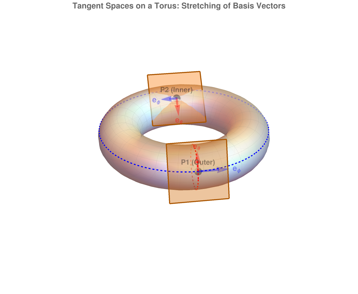
Figure 1.1: Tangent planes to torus. End of Example 1
- Symmetry: gi,j = gj,i (inherited from the symmetry of the inner product).
- Positive Definiteness: For any nonzero vector\( \displaystyle \quad \mathbf{v} = \sum\, v^i \mathbf{e}_i , \quad \langle \mathbf{v} \mid \mathbf{v} \rangle > 0 . \quad \) Consequently, det(G) > 0.
-
Arc Length Element: The infinitesimal squared distance ds² = ⟨dr ∣ dr⟩
is given by the quadratic form:
\[ {\text d}s^2 = \sum_{i=1}^3 \,\sum_{j=1}^3 \,g_{i,j}\, {\text d}q^i \,{\text d}q^j . \]
2. Proof of Positive Definiteness. Let\( \displaystyle \quad \mathbf{v} = \sum_{i=1}^3 \, v^i \,\mathbf{e}_i \quad \) be any nonzero vector in TPℝ³. Using the bilinearity of the inner product, we expand
-
Strict Positivity: Because { e₁, e₂, e₃ }
is a basis, v ≠ 0
if and only if at least one component vⁱ ≠ 0. By the positive-definiteness axiom of the inner product, ⟨v ∣ v⟩ > 0 whenever v ≠ 0. In matrix notation, for any column vector v = [v¹, v², v³]ᵀ ≠ 0:
\[ \mathbf{v}^{\mathrm T} \, G\,\mathbf{v} > 0 . \]
-
Positive Determinant: Because G
is a real, symmetric, positive-definite matrix, all of its eigenvalues λ₁, λ₂, λ₃
are strictly positive (λₖ > 0). Since the determinant of a matrix is the product of its eigenvalues, we conclude:
\[ \det (G) = \lambda_1 \lambda_2 \lambda_3 > 0 . \](Alternative argument via Jacobian: Let\( \displaystyle \quad J = \left[ \frac{\partial x^k}{\partial q^i} \right] \quad \) be the Jacobian matrix of the coordinate transformation. Then\( \displaystyle \quad g_{i,j} = \sum_{k=1}^3 \, \frac{\partial x^k}{\partial q^i} \cdot \frac{\partial x^k}{\partial q^j} , \quad \) , so G = JTJ . Taking determinants gives det(G) = det(JT)·det(J) = (det(J))² > 0 since the coordinate map is locally invertible.)
3. Proof of the Arc Length Element. Consider an infinitesimal displacement dr resulting from small coordinate increments (dq¹, dq², dq³). By the multivariable chain rule (total differential), we expand dr:
Step 1: Compute the Tangent Basis Vectors. Taking partial derivatives of r(u, v, z) gives the natural basis vectors at any point P(u, v, z):
Step 2: Construct the Metric Tensor. (Part 1: Symmetry) Computing all pairwise Euclidean inner products gi,j = ⟨ei ∣ ej⟩:
Step 3: Verify Positive Definiteness (Part 2). Let v = c¹eu + c³ev + c³ez be any tangent vector with components c = [c¹, c², c³]T. Computing the quadratic form cᵀGc:
Step 4: Compute the Arc Length Element (Part 3). Applying Theorem 1(3), the squared infinitesimal distance\( \displaystyle \quad {\text d}s^2 = \sum_{i,j}\, g_{i,j}\,{\text d}q^i\,{\text d}q^j \quad \) is:
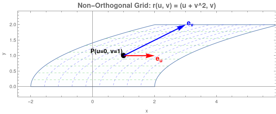
In illustrative plot of the skewed coordinate grid, horizontal green dashed lines represent curves of constant v, while blue dashed parabolas represent curves of constant u. At the point P(u = 0, v = 1) ⇒ (x = 1, y = 1), the tangent vectors eu = (1, 0) and ev = (2, 1) clearly form an acute angle (α &approx 26.6° ≠ 90°), visually explaining why the off-diagonal metric component guv = ⟨eu ∣ ev⟩ = 2v ≠ 0. ■
-
Scale Factors (hi): The lengths of the tangent vectors are defined as
\[ h_i = \| \mathbf{e}_i \| = +\sqrt{\lamgle \mathbf{e}_i \mid \mathbf{e}_i \rangle} = \sqrt{g_{i,i}} . \]
-
Orthonormal Basis: A local orthonormal frame\( \displaystyle \quad \left\{\, \hat{\bf e}_1 , \ \hat{\bf e}_2 , \ \hat{\bf e}_3 \,\right\} \quad \)
is constructed by normalizing the tangent basis:
\[ \hat{\bf e}_i = \frac{\mathbf{e}_i}{h_i} , \qquad i = 1, 2, 3 . \]
- Volume Element: The Jacobian determinant\( \displaystyle \quad J = \det\left( \frac{\partial \mathbf{r}}{\partial q^i} \right) \quad \) satisfies\( \displaystyle \quad J = \sqrt{\det (G)} = h_1 h_2 h_3 , \quad \) yielding the volume element dV = h₁h₂h₃dq¹q²q³.
By definition, a coordinate system is orthogonal at point P if its coordinate curves intersect at right angles, meaning distinct tangent basis vectors are mutually perpendicular:
1. Proof of Scale Factors. In any inner product space, the Euclidean norm (length) of a vector v is induced by the inner product via\( \displaystyle \quad \|\mathbf{v}\| = +\sqrt{\langle \mathbf{v} \mid \mathbf{v}\rangle}. \quad \) Applying this to the i-th tangent basis vector ei yields:
2. Proof of the Orthonormal Basis. Define the normalized vectors\( \displaystyle \quad \hat{\bf e}_i = \frac{1}{h_i}\,\mathbf{e}_i \quad \) for i = 1, 2, 3. Using the bilinearity of the inner product, we compute the pairwise inner products \( \displaystyle \quad \left\langle \mathbf{e}_i \mid \mathbf{e}_j \right\rangle : \)
-
Case i = j: Since gii = (hi)², we obtain:
\[ \left\langle \hat{\bf e}_i \mid \hat{\bf e}_i \right\rangle = \frac{g_{i,i}}{h_i^2} = 1 . \]
-
Case i ≠ j: Since the system is orthogonal,gi.j = 0, so:
\[ \left\langle \hat{\bf e}_i \mid \hat{\bf e}_j \right\rangle = \frac{0}{h_i h_j} = 0 . \]
3. Proof of the Volume Element, Consider an infinitesimal curvilinear coordinate box spanned by the three displacement vectors dr₁ = e₁dq¹, dr₂ = e₂dq², and dr₃ = e₃dq³ (assuming positive increments dqi > 0).
-
Geometric Derivation (via Orthogonality): Because e₁, e₂, e₃
are mutually orthogonal, this infinitesimal parallelepiped is a rectangular box whose edge lengths are:
\begin{align*} {\text d}s_1 &= \| \mathbf{e}_1 \,{\text d}q^1 \| = h_1 \,{\text d}q^1 , \\ {\text d}s_2 &= \| \mathbf{e}_2 \,{\text d}q^2 \| = h_2 \,{\text d}q^2 , \\ {\text d}s_3 &= \| \mathbf{e}_3 \,{\text d}q^3 \| = h_3 \,{\text d}q^3 . \end{align*}The volume of a rectangular box is simply the product of its three orthogonal edge lengths:\[ {\text d}V = {\text d}s_1\,{\text d}x_2 \,{\text d}s_3 = h_1 h_2 h_3 \,{\text d}q^1 \,{\text d}q^2 \,{\text d}q^3 . \]
-
Algebraic Connection to det(G): Recall from multivariable calculus that the volume element is given by the absolute value of the Jacobian determinant, dV = |det(J)| dq¹dq²dq³, where\( \displaystyle \quad J = \left[ \frac{\partial\mathbf{r}}{\partial q^1} \ \frac{\partial\mathbf{r}}{\partial q^2} \ \frac{\partial\mathbf{r}}{\partial q^3} \right]\quad \)
has the tangent vectors ei
as its columns. Since G = JᵀJ
, taking determinants yields:
\[ \det (G) = \det\left( J^{\mathrm T} J \right) = \det\left( J^{\mathrm T} \right) \,\det (J) = (\det J)^2 , \]
- Curves of constant u are confocal ellipses\( \displaystyle \quad \frac{x^2}{a^2\,\cosh^2 u} + \frac{y^2}{a^2\,\sinh^2 u} = 1 \quad \) with foci at (±𝑎, 0).
- Curves of constant v are confocal hyperbolas\( \displaystyle \quad \frac{x^2}{a^2\,\cos^2 v} - \frac{y^2}{a^2\,\sin^2 v} = 1 \quad \) sharing the exact same foci.
Step 1: Natural Tangent Basis Vectors. Taking partial derivatives of r(u, v, z) with respect to u, v, z yields:
- \( \displaystyle \quad \mathbf{e}_u = \frac{\partial\mathbf{r}}{\partial u} = \left( a\,\sinh (u)\, \cos (v) , \ a\,\sinh (u)\,\cos (v) , \ 0 \right) , \)
- \( \displaystyle \quad \mathbf{e}_v = \frac{\partial\mathbf{r}}{\partial v} = \left( -a\,\cosh (u)\,\sin (v) ,\ a\,\sinh (u)\,\cos (v) , \ 0 \right) , \)
- \( \displaystyle \quad \mathbf{e}_z = \frac{\partial\mathbf{r}}{\partial z} = \left( 0, \ 0, \ 1 \right) . \)
Step 2: Verify Orthogonality (gi,j = 0 for i ≠ j).
Computing the off-diagonal inner products:
Dot[D[r[u, v, z], u], D[r[u, v, z], v]]
Step 3: Scale Factors (\( \displaystyle \quad h_i = \sqrt{g_{i,i}} \) ) and Orthonormal Basis.
Computing the diagonal metric components
Taking square roots gives the three scale factors:
Step 4: Volume Element (dV = hu hv hz dudvdz).
Applying Theorem 2(3), the infinitesimal volume element becomes
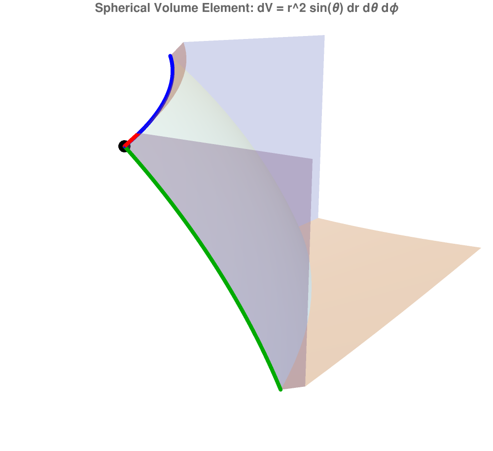
Illustrative Plot: Confocal Ellipses, Hyperbolas, and Orthonormal Frame.
The diagram below shows confocal ellipses (u = constant) and confocal hyperbolas (v = constant) for 𝑎 = 1.5. At P(u₀ = 0.7, v₀ = π/4), the unit vectors\( \displaystyle \quad \hat{\bf e}_u \quad\mbox{and} \quad \hat{\bf e}_v \quad \) are perpendicular and tangent to the intersecting curves.
- Gradient:\( \displaystyle \quad \nabla f = \sum_{i=1}^3 \,\frac{1}{h_i}\,\frac{\partial f}{\partial q^i} \, \hat{\bf e}_i . \)
- Divergence: \( \displaystyle \quad \nabla \bullet \mathbf{F} = \frac{1}{h_1 h_2 h_3} \,\sum_{i=1}^3 \,\frac{\partial}{\partial q^i} \left( \frac{h_1 h_2 h_3}{h_i}\, F_i \right) . \)
- Curl: \( \displaystyle \quad \nabla \times \mathbf{F} = \frac{1}{h_1 h_2 h_3} \,\begin{vmatrix} h_1\,\hat{\bf e}_1 & h_2\,\hat{\bf e}_2 & h_3\,\hat{\bf e}_3 \\ \frac{\partial}{\partial q^1} & \frac{\partial}{\partial q^2} & \frac{\partial}{\partial q^3} \\ h_1 F_1 & h_2 F_2 & h_3 F_3 \end{vmatrix} . \)
- Laplacian: \( \displaystyle \quad \nabla^2 f = \frac{1}{h_1 h_2 h_3} \,\sum_{i=1}^3 \,\frac{\partial}{\partial q^i} \left( \frac{h_1 h_2 h_3}{h_i}\, \frac{\partial f}{\partial q^i} \right) . \)
By the coordinate-free definition of the gradient, ∇ f, is the unique vector field satisfying df = ⟨∇f , dr⟩ for every infinitesimal displacement dr.
Expand ∇f in the local orthonormal basis as\( \displaystyle \quad \nabla f = c_1 \hat{\bf e}_1 + c_2 \hat{\bf e}_2 + c_3 \hat{\bf e}_3 . \quad \) From Theorem 2, the infinitesimal displacement vector is\( \displaystyle \quad {\text d}\mathbf{r} = \sum_{i=1}^3 \,h_i {\text d}q^i \hat{\bf e}_i . \quad \) Taking the inner product gives:
Preliminary Lemma for Divergence and Curl.
Applying Part 1 to each coordinate function f = qi gives:
2. Proof of the Divergence.
Using the lemma above, write the first component of F
as:
3. Proof of the Curl.
Using\( \displaystyle \quad \hat{\bf e}_1 = h_1 \nabla q^1 , \quad \)
, rewrite the first term of F
as\( \displaystyle \quad F_1 \hat{\bf e}_1 = \left( h_1 F_1 \right) \nabla q^1 . \quad \) Apply the vector product rule ∇ × (ϕA) = *nabla;ϕ × A + ϕ(∇ × A) with ϕ = h₁F₁ and A = ∇q¹. Since ∇ × ∇q¹ = 0, this simplifies to:
4. Proof of the Laplacian.
By definition, the scalar Laplacian is the divergence of the gradient: &nabla²f = ∇ • (∇f). Set F = ∇f, whose components from Part 1 are:
Note: Classical textbooks often prove divergence and curl using flux integrals over infinitesimal boxes and circulation around infinitesimal loops (requiring careful Taylor expansions on opposite faces). Using the coordinate gradients makes the proof purely algebraic, exact, and free of higher-order remainder terms.
- Coordinate Geometry: Surfaces of constant σ and τ are orthogonal families of confocal parabolic cylinders opening upward and downward along the y-axis.
-
Scale Factors (from Theorem 2): Computing \( \displaystyle \quad h_i = \left\| \frac{\partial\mathbf{r}}{\partial q^i} \right\| \quad \)
gives non-constant, coupled scale factors:
\[ h_{\sigma} = \sqrt{\sigma^2 + \tau^2} , \quad h_{\tau} = \sqrt{\sigma^2 + \tau^2} , \quad h_z = 1 . \]Notice that hσhτhz = σ² + τ².
Part 1: Gradient and Laplacian of a Scalar Field.
Consider the scalar potential field f(σ, τ, z) = σ²τ + z².
-
Gradient (∇f):
Applying Theorem 3(1):
\[ \nabla f = \frac{1}{h_{\sigma}}\, \frac{\partial f}{\partial\sigma}\, \hat{\bf e}_{\sigma} + \frac{1}{h_{\tau}}\, \frac{\partial f}{\partial\tau}\, \hat{\bf e}_{\tau} + \frac{1}{h_z}\, \frac{\partial f}{\partial z} \,\hat{\bf e}_z . \]Substituting the partial derivatives \( \displaystyle \quad \frac{\partial f}{\partial\sigma} = 2\sigma\tau , \quad \frac{\partial f}{\partial\tau} = \sigma^2 , \quad \mbox{and} \quad \frac{\partial f}{\partial z} = 2z \quad \) yields:\[ \nabla f = \frac{2\sigma\tau}{\sqrt{\sigma^2 + \tau^2}}\, \hat{\bf e}_{\sigma} + \frac{\sigma^2}{\sqrt{\sigma^2 + \tau^2}}\, \hat{\bf e}_{\tau} + 2z\,\hat{\bf e}_z . \]
-
Laplacian (∇²f):
Applying Theorem 3(4), notice how the scale-factor ratios \( \displaystyle \quad \frac{h_\tau h_z}{h_\sigma} = 1 \quad\mbox{and} \quad \frac{h_\sigma h_z}{h_\tau} = 1 \quad \) simplify the inner derivatives, while \( \displaystyle \quad \frac{h_\sigma h_\tau}{h_z} = \sigma^2 + \tau^2 : \)\[ \nabla^2 f = \frac{1}{\sigma^2 + \tau^2} \left[ \frac{\partial}{\partial\sigma} \left( 1 \cdot 2\sigma\tau \right) + \frac{\partial}{\partial \tau} \left( 1 \cdot \sigma^2 \right) + \frac{\partial}{\partial z} \left(\left( \sigma^2 + \tau^2 \right) \cdot 2z \right) \right] . \]Evaluating each derivative gives:\[ \nabla^2 f = \frac{2\tau}{\sigma^2 + \tau^2} + 2 . \]
Consider a swirling, radially expanding vector field expressed directly in the local orthonormal basis \( \displaystyle \quad \left\{ \hat{\bf e}_\sigma , \ \hat{\bf e}_\tau , \ \hat{\bf e}_z \right\} : \)
-
Divergence (∇ • F):
Applying Theorem 3(2), the scale-factor products inside the derivatives simplify cleanly:\[ F_{\sigma} h_\tau h_z = \sigma , \quad F_{\tau} h_\sigma h_z = \tau , \quad F_z h_\sigma h_\tau = \sigma\tau \left( \sigma^2 + \tau^2 \right) . \]Substituting these into the divergence formula gives:\begin{align*} \nabla \bullet \mathbf{F} &= \frac{1}{\sigma^2 + \tau^2} \left[ \frac{\partial}{\partial\sigma} \left( \sigma \right) + \frac{\partial}{\partial\tau} \left( \tau \right) + \frac{\partial}{\partial z}\left( \sigma\tau \left( \sigma^2 + \tau^2 \right) \right) \right] \\ &= \frac{}{\sigma^2 + \tau^2} . \end{align*} -
Curl (∇ × F):
Applying Theorem 3(3), compute the scaled components hiFi:\[ h_\sigma F_{\sigma} = \sigma , \quad h_\tau F_\tau = \tau , \quad h_z F_z = \sigma \tau . \]Expanding the determinant:\[ \nabla \times \mathbf{F} = \frac{1}{\sigma^2 + \tau^2} \begin{vmatrix} \sqrt{\sigma^2 + \tau^2}\,\hat{\bf e}_\sigma & \sqrt{\sigma^2 + \tau^2}\,\hat{\bf e}_\tau & \hat{\bf e}_z \\ \frac{\partial}{\partial \sigma} & \frac{\partial}{\partial \tau} &\frac{\partial}{\partial z} \\ \sigma & \tau & \sigma\tau \end{vmatrix} . \]Evaluating each component of the determinant yields:- \( \displaystyle \quad \hat{\bf e}_\sigma \quad \) component: \( \displaystyle \quad \frac{\sqrt{\sigma^2 + \tau^2}}{\sigma^2 + \tau^2} \left( \frac{\partial}{\partial \tau} \left( \sigma \right) - \frac{\partial}{\partial z} \left( \sigma\tau \right) \right) = \frac{\sigma}{\sqrt{\sigma^2 + \tau^2}} . \)
- \( \displaystyle \quad \hat{\bf e}_\tau \quad \) component: \( \displaystyle \quad \frac{\sqrt{\sigma^2 + \tau^2}}{\sigma^2 + \tau^2} \left( \frac{\partial}{\partial z} \left( \sigma \right) - \frac{\partial}{\partial \sigma} \left( \sigma\tau \right) \right) = - \frac{\tau}{\sqrt{\sigma^2 + \tau^2}} . \)
- \( \displaystyle \quad \hat{\bf e}_z \quad \) component: \( \displaystyle \quad \frac{1}{\sigma^2 + \tau^2} \left( \frac{\partial}{\partial z} \left( \tau \right) - \frac{\partial}{\partial \tau} \left( \sigma \right) \right) = 0 . \)
\[ \nabla \times \mathbf{F} = \frac{\sigma}{\sqrt{\sigma^2 + \tau^2}}\, \hat{\bf e}_\sigma - \frac{\tau}{\sqrt{\sigma^2 + \tau^2}}\, \hat{\bf e}_\tau . \]
| Coordinate System | Transformation $\mathbf{r}(q^1, q^2, q^3)$ | Metric Tensor $G = \operatorname{diag}(g_{11}, g_{22}, g_{33})$ | Scale Factors $(h_1, h_2, h_3)$ |
|---|---|---|---|
| Cylindrical $(\rho, \phi, z)$ |
$x = \rho\cos\phi$ $y = \rho\sin\phi$ $z = z$ |
$\operatorname{diag}(1, \rho^2, 1)$ | $(1, \rho, 1)$ |
| Spherical $(r, \theta, \phi)$ |
$x = r\sin\theta\cos\phi$ $y = r\sin\theta\sin\phi$ $z = r\cos\theta$ |
$\operatorname{diag}(1, r^2, r^2\sin^2\theta)$ | $(1, r, r\sin\theta)$ |
| Elliptic Cylindrical $(\mu, \nu, z)$ |
$x = a\cosh\mu\cos\nu$ $y = a\sinh\mu\sin\nu$ $z = z$ |
$\operatorname{diag}\big(a^2(\sinh^2\mu + \sin^2\nu),\, a^2(\sinh^2\mu + \sin^2\nu),\, 1\big)$ | $(h, h, 1)$ where $h = a\sqrt{\sinh^2\mu + \sin^2\nu}$ |
- Vector addition
- Brannon, R.M., Curvilinear Analysis in a Euclidean Space, Utah, 2004.
- Curvilinear coordinates