
Introduction to Linear Algebra
Systems of Linear Equations
- Introduction
- Linear systems
- Vectors
- Linear combinations
- Matrices
- Planes in ℝ³
- Equation A x = b
- Sensitivity of solutions
- Linear independence
- Plane transformations
- Space transformations
- Linear transformations
- Affine maps
- Exercises
- Answers
Matrix Algebra
- Introduction
- Manipulation of matrices
- Partitioned matrices
- Block matrices
- Matrix operators
- Determinants
- Cofactors
- Cramer's rule
- Chiò's method
- Equivalent matrices
- Elimination: A = L U
- PLU factorization
- Reflection
- Givens rotation
- Special matrices
- Exercises
- Answers
Vector Spaces
- Introduction
- Motivation
- Vector spaces
- Bases
- Dimension
- Coordinate systems
- Linear transformations
- Change of basis
- Matrix transformations
- Compositions
- Isomorphisms
- Dual transformations
- Quotient spaces
- Wedge products
- Rotors
Eigenvalues, Eigenvectors
- Introduction
- Characteristic polynomials
- Companion matrix
- Algebraic and geometric multiplicities
- Minimal polynomials
- Eigenspaces
- Where are eigenvalues?
- Eigenvalues of A B and B A
- Generalized eigenvectors
- Similarity
- Diagonalizability
- Self-adjoint operators
- Exercises
- Answers
Euclidean Spaces
- Introduction
- Euclidean space
- Bilinear transformations
- Norm and distance
- Matrix norms
- Dual norms
- Dual transformations
- Examples of transformations
- Orthogonality
- Gram--Schmidt Process
- Orthogonal matrices
- Self-adjoint matrices
- Unitary matrices
- Projection operators
- QR-decomposition
- Least Square Approximation
- Quadratic forms
- Exercises
- Answers
Canonical forms
- Introduction
- 2D decomposition
- 3D decomposition
- Projectors
- Direct-sum decompositions
- Cyclic decompositions
- Symmetric matrices
- Symmetric matrices
- Pseudoinverse
- URV-decomposition
- LU-decomposition
- PLU-decomposition
- QR-decomposition
- Cholesky decomposition
- Schur decomposition
- Positive matrices
- Roots
- Polar factorization
- Spectral decomposition
- CUR decomposition
- Exercises
- Answers
Applications
- Introduction
- Circles along curves
- TNB frames
- GPS problem
- Coriolis acceleration
- Poisson equation
- Graph theory
- Error correcting codes
- Electric circuits
- FSA
- Markov chains
- Cryptography
- Wave-length transfer matrix
- Computer graphics
- Linear Programming
- Hill's determinant
- Fibonacci matrices
- Discrete dynamic systems
- Discrete Fourier transform
- Fast Fourier transform
- Curve fitting
- Answers
Miscellany
- Introduction
- Circles along curves
- TNB frames
- Differential forms
- Calculus
- Vector representations
- Matrix representations
- Change of basis
- Orthonormal Diagonalization
- Generalized inverse
- Differential forms
Preliminaries
- Complex Number Operations
- Sets
- Polynomials
- Polynomials and Matrices
- Computer solves Systems of Linear Equations
- Location of Eigenvalues
- Power Method
- Iterative Method
- Similarity and Diagonalization
Glossary
Reference

This Book is licensed under Creative Commons Attribution-NonCommercial-NoDerivs 3.0 Unported License
The Wolfram Mathematica notebook which contains the code that produces all the Mathematica outputs in this web page may be downloaded at this link. Caution: This notebook will evaluate, cell-by-cell, sequentially, from top to bottom. However, due to re-use of variable names in later evaluations, computer memory must be cleared with command Clear[ ] prior further code execution.
Remove[ "Global`*"] // Quiet (* remove all variables *)
Linear algebra is primarily concerned with two types of mathematical objects: vectors and their transformations or matrices. Moreover, these objects are common in all branches of science related to physics, engineering, economics, and through computer technologies to almost all branches of science. Since matrices are build from vectors, this section focuses on the latter by presenting basic vector terminology and corresponding concepts. Fortunately, we have proper symbols for their computer manipulations.
There are two approaches in science literature to define vectors---one is abstract, especially those on linear algebra texts (you will meet it in part 3 of this tutorial), another trend involving engineering and physics topics is based on geometrical interpretation or coordinates definition, caring sequences of numbers. Computer science folks sit on both chairs because they utilize both interpretations of vectors. Moreover, they introduced abstract analogues of vectors---lists and arrays are widely used in mathematical books. We all observe a shift in science made by computer science including impact on classical mathematics.
Vectors
What is a vector? It turns out that the answer depends on who is asking. In classical mechanics and calculus, you learn that a vector is a mathematical object that has both magnitude (or length) and direction. In quantum mechanics, you will discover that instead of geometrical definition of vectors, you need to know more abstract objects, called bra- and ket-vectors. Studying functional analysis, integral equations, and partial differential equations you meet with special kind of vectors, called covectors or functionals. Later, when you want to understand what Albert Einstein contributed to the world, you discover two types of vectors: covariant vectors and contravariant vectors. In graduate study, you will meet three types of vectors in Machine Learning course: feature vectors, thought vectors, and word vectors.In the third chapter of this tutorial, you will learn how all these different kinds of vector definition can be united into one mathematically well-motivated generalization. This section is devoted to one particular version of vectors that is closely related to solving systems of linear equations. Moreover, it establishes a connection of our algebraic definition of vectors with similar definition of vectors in object oriented computer languages such as C++ that generalize such terms as arrays and lists.
Mathematicians distinguish between vector and scalar (pronounced “SKAY-lur”) quantities. You’re already familiar with scalars—scalar is the technical term for an ordinary number. In this course, we use four specific sets of scalars: integers ℤ, rational numbers ℚ, real numbers ℝ, and complex numbers ℂ. We abbreviate these four sets with symbol 𝔽 (which is either ℤ or ℚ or ℝ or ℂ). Be aware that we do not cover the seemingly exotic finite fields only for technical reasons; however, they are very important in some applications (see for example, in coding theory). By a vector we mean a list or finite sequence of numbers. We employ scalars when we wish to emphasize that a particular quantity is not a vector quantity. For example, as we will discuss shortly, “velocity” and “displacement” are vector quantities, whereas “speed” and “distance” are scalar quantities.
In this section, we focus on algebraic definition of vectors as arrays of numbers and put its geometrical interpretation on back burner (Part 3).
It wasn’t until the early 1600s that thermometer began to come into its own. The famous Italian astronomer and physicist Galileo Galilei (1564--1642), or possibly his friend the physician Santorio, likely came up with an improved thermoscope around 1593: An inverted glass tube placed in a bowl full of water or wine. Santorio apparently used a device like this to test whether his patients had fevers. Shortly after the turn of the 17th century, English physician Robert Fludd also experimented with open-air wine thermometers.
The first recorded instance of anyone thinking to create a universal scale for thermoscopes was in the early 1700s. In fact, two people had this idea at about the same time. One was a Danish astronomer named Ole Christensen Rømer (1644--1710), who had the idea to select two reference points—the boiling point of water and the freezing point of a saltwater mixture, both of which were relatively easy to recreate in different labs—and then divide the space between those two points into 60 evenly spaced degrees. The other was England’s revolutionary physicist and mathematician Isaac Newton (1643--1727), who announced his own temperature scale, in which 0 was the freezing point of water and 12 was the temperature of a healthy human body, the same year that Rømer did. (Newton likely developed this admittedly limited scale to help himself determine the boiling points of metals, whose temperatures would be far higher than 12 degrees.)
After a visit to Rømer in Copenhagen, the Dutch-Polish physicist Daniel Fahrenheit (1686--1736) was apparently inspired to create his own scale, which he unveiled in 1724. His scale was more fine-grained than Rømer’s, with about four times the number of degrees between water’s boiling and freezing points. Fahrenheit is also credited as the first to use mercury inside his thermometers instead of wine or water. Though we are now fully aware of its toxic properties, mercury is an excellent liquid for indicating changes in temperature.
Originally, Fahrenheit set 0 degrees as the freezing point of a solution of salt water and 96 as the temperature of the human body. But the fixed points were changed so that they would be easier to recreate in different laboratories, with the freezing point of water set at 32 degrees and its boiling point becoming 212 degrees at sea level and standard atmospheric pressure.
But this was far from the end of the development of important temperature scales. In the 1730s, two French scientists, Rene Antoine Ferchault de Réamur (1683--1757) and Joseph-Nicolas Delisle (1688--1768), each invented their own scales. Réamur’s set the freezing point of water at 0 degrees and the boiling point of water at 80 degrees, convenient for meteorological use, while Delisle chose to set his scale “backwards,” with water’s boiling point at 0 degrees and 150 degrees (added later by a colleague) as water’s freezing point.
A decade later, Swedish astronomer Anders Celsius (1701--1744) created in 1742 his eponymous scale, with water’s freezing and boiling points separated by 100 degrees—though, like Delisle, he also originally set them “backwards,” with the boiling point at 0 degrees and the ice point at 100. (The points were swapped after his death.) In 1745, Carolus Linnaeus (1707--1778) of Uppsala, Sweden, suggested that things would be simpler if we made the scale range from 0 (at the freezing point of water) to 100 (water’s boiling point), and called this scale the centigrade scale. (This scale was later abandoned in favor of the Celsius scale, which is technically different from centigrade in subtle ways that are not important here.) Notice that all of these scales are relative—they are based on the freezing point of water, which is an arbitrary (but highly practical) reference point. A temperature reading of x°C basically means “x degrees hotter than the temperature at which water freezes.”
Then, in the middle of the 19th century, British physicist William Lord Kelvin (1824--1907) also became interested in the idea of “infinite cold” and made attempts to calculate it. In 1848, he published a paper, On an Absolute Thermometric Scale, that stated that this absolute zero was, in fact, -273 degrees Celsius. (It is now set at -273.15 degrees Celsius.)
Loudness:
Loudness is usually measured in decibels (abbreviated dB). To be more precise, decibels are used to measure the ratio of two power levels. If we have two power levels P₁ and P₂, then the difference in decibels between the two power levels is \[ 10\,\log_{10} \left( \frac{P_2}{P_1} \right) \ \mbox{dB} . \] So, if P₂ is about twice the level of P₁, then the difference is about 3 dB. Notice that this is a relative system, providing a precise way to measure the relative strength of two power levels, but not a way to assign a number to one power level.Note that humans perceive loudness based on the intensity (amplitude) of sound waves, but also taking into account frequency and duration. While the ear converts sound waves into electrical signals that the brain interprets, loudness is a subjective experience influenced by factors beyond simple sound pressure level. While decibels (dB) measure sound intensity objectively, perceived loudness is subjective and doesn't increase linearly with decibel increases.
The generally accepted just noticeable difference (JND) in sound intensity for the average human ear is approximately 1 dB. This means that, on average, a change of about 1 dB is the smallest difference in loudness that a typical listener can reliably detect. However, under ideal, quiet conditions with pure tones and focused attention, some people can detect differences as small as 0.5 dB. In particular, the difference of +3 dB: is barely perceptible — this is often considered the minimum noticeable difference in loudness in sound level that is clearly noticeable in typical settings like music or speech. +5 dB: is clearly audible change; +10 dB: is perceived as twice as loud; +20 dB: is perceived as four times as loud.
These two examples of scalars (temperature and loudness) show that mother nature put bounds (upper and lower) of their applications in real life. Even in possible future, people may use another scaling in enumeration of these scalars, they still will be bounded. From mathematical prospective, it is not convenient to be restricted in calculations with these scalars or numbers. Therefore, mathematicians use their lovely trick (crucial concept) discovered in the seventeen century with calculus invention---infinity (or limit, which is equivalent). So the set of all real numbers, denoted by ℝ, is called a scalar set and our two examples constitute only a part of ℝ, but not the whole set of scalars (which must be unbounded by definition). ■
Vectors and Points
Points and vectors, while often related, represent different concepts. There is a special mathematical structure that treats them strictly differently---affine space. A point indicates a specific location in space, while a vector represents a displacement or direction with magnitude (length). Since vectors have no fixed position in space, they sometimes are called free vectors. A vector starting at the origin and having its tip at particular point is called a coordinate vector. Geometrically, we draw points as dots and vectors as line segments with arrows.
Besides that we can add or subtract vectors, we can also add a vector to a point to get another point. This gives us a way to describe points. We need to have a starting point (the origin). We can then represent any point in space by the vector that connects the origin to that point. In this sense, each point corresponds uniquely to a position vector anchored at the origin. This identification establishes a bijection (one-to-one and onto correspondence) between points and vectors. When origin and frame are established, both vectors and points can be described as an array of numbers.
Note that the set-builder notation admits separation of sets and their properties by either two vertical dots or vertical line. Remember that order of pairing sets A and B in its Cartesian product A × B matters. For instance, if ℤ = {0, ±1, ±2, …} is paired with itself, the ordered pairs (1, 3) and (3, 1) represent distinct elents from ℤ × ℤ, but the sets {3, 1} and {1. 3} are equal. The arrays (2, 2) and (2, 2, 2) are not equal (they do not have the same length), although the sets {2, 2} and {2, 2, 2} both equal the set {2}.
This definition can be extended for arbitrary finite number of sets, forming an n-fold Cartesian product. Although mathematician define Cartesian products for arbitrary family of sets, we do not use it in this tutorial.
An important special case is a power of an object 𝑋, where we take all 𝑋j to be 𝑋 and form \( \displaystyle \quad X^J = \prod_{j\in J} X . \quad \) When J is the finite set of integers, [1..n] = {1, 2, … , n}, the n-fold Cartesian product of set X is \( \displaystyle \quad X^{[1..n]} . \)
Given sets A₁, A₂, etc., the Cartesian product of the countably infinitary family (A₁, A₂, … ) is written as \( \displaystyle \quad \prod_{j=1}^{\infty} A_j ; \quad \) its elements (𝑎₁, 𝑎₂, 𝑎₃, …) are called infinite sequences.
The Cartesian product of the empty family () is the point, a set whose only element is the empty list ().
In categories of algebras, products are constructed in the “obvious” manner; see for example direct product group.
An n-tuple is an ordered list of n elements, which are typically enclosed in parentheses to represent points in n-dimensional space. Strictly speaking, n-tuples are not vectors but points because they are elements of the Cartesian product 𝔽[1..n] and as so there is not vector structure. Points cannot be added as pixels on your screen, but you can add (or attach) a vector to a point and obtain a new point. It will be shown shortly that the corresponding space of points can be equipped with addition and scalar multiplication that makes it a vector space. In many textbooks, n-tuples are identified with vectors keeping in mind corresponding isomorphism between points and vectors.
If you have ever played chess, you have some exposure to two dimensional (2D) Cartesian coordinate spaces. A chessboard is usually enumerated with a system called algebraic notation. Each square is identified by a letter (a-h) for the file (column) and a number (1-8) for the rank (row), from the perspective of the white player. So white king is initially in position A5. This creates a grid of 64 unique squares, like a coordinate system on the board.
It is possible to use the Cartesian product [1..8](a-h) for enumeration of squares in the chessboard. So white king will be initially in position E1; However, such enumeration is not used in practice. ■
The following example demonstrates a practical application of two dimensional Cartesian product to possible planning of streets in a city.
Let’s imagine a fictional city named Cartesia. Inspired by Manhattan, a borough of New York City, the Cartesia city planners were laying out the streets and avenues in a very particular way, as illustrated in the map of Cartesia in Figure 3.1. As you can see from the map, Center Avenue runs east-west through the middle of town. All other east-west avenues (parallel to Center Avenue) are named based on whether they are north or south of Center Avenue, and how far they are from Center Avenue. Examples of avenues that run east-west are North 3rd and South 15th Avenue.
The other streets in Cartesia run north. Division Street runs north-south through the middle of town. All other north-south streets (parallel to Division Street) are named based on whether they are east or west of Division Street, and how far they are from Division Street.
Of course, the map of Cartesia is an idealization of rectangular plane---there is no limit in space of the Cartesian space, and streets do not have width being drawn through any point. Nevertheless, this map shows coordinate lines parallel to abscissa (streets) and ordinate (avenues).
■As you know, a point has a location but no real size or thickness. In order to identify position of a point, we need to establish a global frame relative to which we specify location of a point. However, an “absolute” position does not exist. For instance, any position on the earth can be specified by its latitude, longitude, and height above sea level.
Every attempt to describe a position requires that we describe it relative to something else. Any description of a position is meaningful only in the context of some (typically “larger”) reference frame. Theoretically, we could establish a reference frame encompassing everything in existence and select a point to be the “origin” of this space, thus defining the “absolute” coordinate space. Luckily for us, absolute positions in the universe aren’t important. Do you know your precise position in the universe right now?
In many cases, displacements are from the origin, and so there will be no distinction between points and vectors because they both share the same coordinates. However, we often deal with quantities that are not relative to the origin, or any other point for that matter. In these cases, it is important to visualize these quantities as an arrow rather than a point.
We consider points as elements of Cartesian product 𝔽[1..n] of n scalar fields. Then every point P from ℝ[1..n] has n coordinates that specify its position:
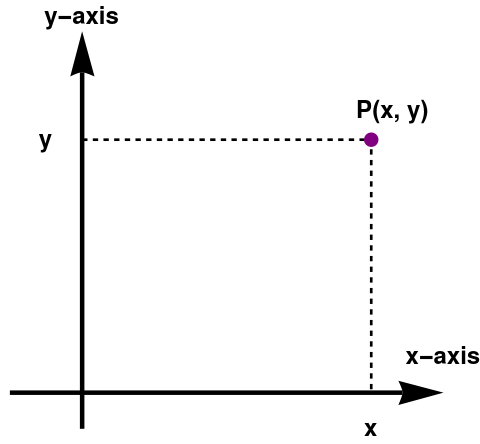
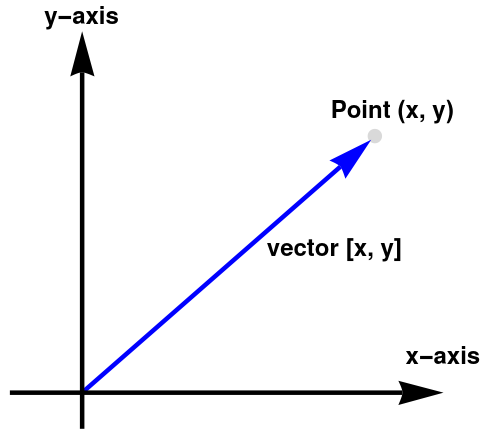
Since positions are relative to some larger frame, points are relative as well— they are relative to the origin of the coordinate system used to specify their coordinates. This leads us to the relationship between points and vectors. The following figure illustrates how the point (x, y) is related to the vector [x, y], given arbitrary values for x and y.
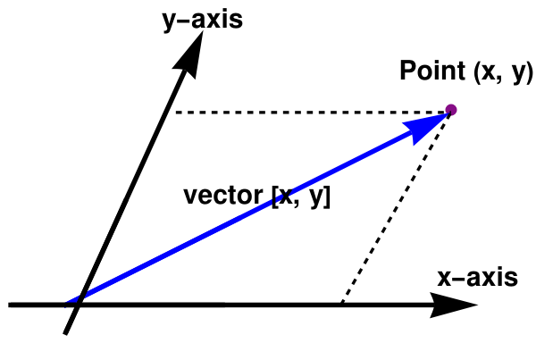
Be aware that Figure 2 is not 100% accurate because a vector space has no property to identify which vector is perpendicular to another vector as we plotted coordinate axes. To define the orthogonality of vectors, one needs to impose additional structure into the vector space (in this case, this space is called an Euclidean space, see Chapter 5). The following figure shows the relationship between points and vectors in oblique coordinate system.
As you see, we use lower case bold font to denote vectors. In opposite to vectors, we denote points by upper case letters in italic font. Since every multiple ℝ in ℝ[1..n] is a real line containing all real numbers in natural order, every element of the Cartesian product is uniquely identified by a list of n numbers, which we call a point. Vectors are used to describe displacements, and therefore they can describe relative positions. Points are used to specify positions.
Every point on the plane has two coordinates P(x, y) relative to the origin of the coordinate system. This point can also be identified by a vector pointed to it and started from the origin. This means that the vector also can be uniquely identified by the same pair v = [x, y]. This establishes a one-to-one correspondence between points and vectors.
Vectors as elements of 𝔽n
The Cartesian product deals with sets. However, we would like to extend it to fields rather than sets. Since fields possess an algebraic structure—defined by two operations, addition and multiplication---we would like to extend these operations to elements of Cartesian products. The following construction demonstrates how the Cartesian product 𝔽[1..n] of n scalar fields can be transferred into a vector space by introducing arithmetic operations inherited from the scalar field.
It was G.W. Leibniz (1646--1716) who first called them "coordinates." REcall that [1..n] = {1, 2, … , n is the set of first n natural numbers.
It was a Welsh physician and mathematician Robert Recorde (1510--1558) who invented the equal sign (=) circa 1557 and also introduced the pre-existing plus (+) and minus (−) signs to English speakers in 1557.
When we wish to refer to the individual components in a vector, we use subscript notation. In math literature, integer indices are used to access the elements of n-tuple. As it follows from the definition above, vectors can be added/subtracted and multipled by a scalar.
Computational technologies allow languages to be treated like vector spaces with precise mathematical properties. Let us consider four words as vectors of the same size: \[ {\bf King}, \quad {\bf Queen}, \quad {\bf man}, \quad {\bf woman}. \] We can write a linear equation that makes sense: \[ {\bf King} - {\bf man} + {\bf woman} = {\bf Queen} . \] You can interchange the order of words in the left-hand side as, for instance, \[ {\bf King} + {\bf woman} - {\bf man} = {\bf Queen} . \]
People generally know and use thousands of words; on average, working males use 2000-3000 words, females from 10,000-20000.
Matrix forms of vectors
Computers store matrices as a single, one-dimensional array of numbers, along with metadata that indicates the matrix's dimensions (number of rows and columns). This structure is computationally efficient for storage and access of matrix elements using their row and column indices. Different languages and libraries might use row-major or column-major ordering to map the 2D matrix to the 1D array. Therefore, computers treat matrices as one-dimensional arrays (actually vectors) with some auxiliary instructions containing two numbers: m, the number of rows, and n, the number of columns.
The dimension of a vector tells us how many numbers the vector contains; it is n when a vectors is taken from 𝔽n. Vectors may be of any positive dimension, including one. In fact, a scalar can be considered a one dimensional (1D for short) vector. . When writing a vector from 𝔽n, mathematicians list the numbers surrounded by parentheses:
Finally, we consider diagonal matrices
a == b
Lists vs arrays vs vectors
Information technologies affect many traditional branches of science including mathematics. Programming languages and their applications constantly lead to updates of regular terms by adding some properties as well as introducing new ones. Now we observe that computer science terminology penetrates mathematical language, especially discrete mathematics and numerical analysis. Moreover, existing computational solvers dictate standardization of terminology in a new way making some notations and terms obsolescence. For example, more and more mathematicians follow the computer genius and inventor of new terms Donald Knuth and replace the Pochhammer symbol with rising factorial.
In many textbooks on Linear Algebra, you may find such terms as "list" or "array" as synonymous of the familiar word "vector" because there is no universally accepted definitions of these terms. Be aware that these terms are used in different computer languages and they may have different options. Array's definition does not allow to change its size and datatype.
The term vector appears in a variety of mathematical and engineering contexts, which we will discuss in Part3 (Vector Spaces). There is no universal notation for vectors because of diversity of their applications. Until then, vector will mean an ordered set (list) of numbers. Generally speaking, concept of vector may include infinite sequence of numbers or other objects. However, in this part of tutorial, we consider only finite lists.
In the context of algorithm analysis, a list is a fundamental data structure that represents a collection of elements in a specific order. It is a linear collection where each element is stored at a position, and these positions are arranged sequentially. Lists can be implemented using various techniques, such as arrays or linked structures.
Array and list are data structures that are used to store the data in a specific order, such as a list of student names or a sequence of numbers, while lists are mutable, meaning that they can be changed after they are created. Arrays are more memory efficient than lists for storing large collections of data of the same type. Arrays are mutable, meaning you can modify their content after creation. However, the type of elements they store remains consistent.
While arrays and vectors are mutable, their size is not as dynamically adjustable as lists. However, you can still append, extend, or remove elements from arrays and vectors, but it will result in a new array or vector of different size. Hence, list is appropriate to store student's names because lists can grow or shrink in size dynamically. You can cotenate it with any number of students who want to join your course. Similarly, when students drop the course, you just delete their names without changing the file name.
An array is always of a fixed size; it does not grow as more elements are required. The programmer must ensure that only valid values in the array are accessed, and must remember the location in the array of each value. Arrays are basic types in most programming languages and have a special syntax for their use.
Vectors are much like arrays, but data in their entries can be of distinct type. Unlike static arrays, which are always of a fixed size, vectors can be grown. This can be done either explicitly or by adding more data, which leads to new vectors.
In most functional programming languages, the word list always refers to a linked list built out of pairs, where each pair contains one list element and a pointer to the next pair. Whereas a list is built out of out of interlinked but still separate objects, a vector is a single object.
Recall that lists can be made of any type of element. A list element can also be a list. For example: [2, [3, 5], 17] is a valid list with the list [3, 5] being the element at index 2. When a list is an element inside a larger list, it is called a nested list.
Mathematica also has a special command Array
Vector Properties
For dimensions greater than three, we can no longer rely on visual representations of vectors. Therefore, it's essential to develop the ability to manipulate and calculate vectors algebraically, much like we do with real numbers. In many cases, vector operations resemble those of scalar arithmetic, and familiar algebraic rules apply. However, as we progress, we will encounter situations where vector algebra behaves quite differently from our experience with real numbers. For this reason, it's crucial to verify any algebraic properties before applying them.
The following theorem summarizes the main properties of vectors from the direct product 𝔽n for any positive integer n. Later in part 3 of this tutorial, you will see that these properties are valid for arbitrary vector spaces. The word "theorem" is derived from the Greek word "theorema," which in turn comes from a word meaning "to look at."
- u + v = v + u,
- (u + v) + w = u + (v + w),
- u + 0 = u,
- u + (−u) = 0,
- α (u + v) = α u + α v,
- (α + β) u = α u + β u,
- α (βu) = (αβ) u,
- 1·u = u.
- \begin{align*} \mathbf{u} + {\ng v} &= \begin{pmatrix} u_1 & u_2 & \cdots & u_n \end{pmatrix} + \begin{pmatrix} v_1 & v_2 & \cdots & v_n \end{pmatrix} \\ &= \begin{pmatrix} u_1 + v_1 & u_2 + v_2 & \cdots & u_n + v_n \end{pmatrix} \\ &= \begin{pmatrix} v_1 + u_1 & v_2 + u_2 & \cdots ( v_n + u_n \end{pmatrix} \\ &= \mathbf{v} + {\bf u} \end{align*}
- \begin{align*} \left( \mathbf{u} + \mathbf{v} \right) + \mathbf{w} &= \left( \begin{pmatrix} u_1 & u_2 & \cdots & u_n \end{pmatrix} + \begin{pmatrix} v_1 & v_2 & \cdots & v_n \end{pmatrix} \right) \\ & \quad + \begin{pmatrix} w_1 & \cdots & w_n \end{pmatrix} \\ &= \begin{pmatrix} u_1 + v_1 & u_2 + v_2 & \cdots & u_n + v_n \end{pmatrix} \\ & \quad + + \begin{pmatrix} w_1 & \cdots & w_n \end{pmatrix} \\ &= \begin{pmatrix} u_1 + v_1 + w_1 & u_2 + v_2 + w_2 & \cdots & u_n + v_n + w_n \end{pmatrix} \\ &= \begin{pmatrix} u_1 & u_2 & \cdots & u_n \end{pmatrix} \\ & \quad + \begin{pmatrix} v_1 + w_1 & v_2 + w_2 & \cdots & v_n + w_n \end{pmatrix} \\ &= \mathbf{u} + \left( \mathbf{v} + \mathbf{w} \right) . \end{align*}
- \begin{align*} \mathbf{u} + \mathbf{0} &= \begin{pmatrix} u_1 & u_2 & \cdots & u_n \end{pmatrix} + \begin{pmatrix} 0&0& \cdots & 0 \end{pmatrix} \\ &= \begin{pmatrix} u_1 + 0 & u_2 + 0 & \cdots & u_n + 0 \end{pmatrix} \\ &= \begin{pmatrix} u_1 & u_2 & \cdots & u_n \end{pmatrix} \\ &= \mathbf{u} . \end{align*}
- \begin{align*} \mathbf{u} + \left( - \mathbf{u} \right) &= \begin{pmatrix}u_1 & u_2 & \cdots & u_n \end{pmatrix} \\ &\quad - \begin{pmatrix} u_1 & u_2 & \cdots & u_n \end{pmatrix} \\ &= \begin{pmatrix}u_1 & u_2 & \cdots & u_n \end{pmatrix} \\ &\quad + \begin{pmatrix} -u_1 & -u_2 & \cdots & -u_n \end{pmatrix} \\ &= \begin{pmatrix}u_1 - u_1 & u_2 - u_2 & \cdots & u_n - u_n \end{pmatrix} \\ &= \begin{pmatrix} 0&0& \cdots & 0 \end{pmatrix} = \mathbf{0} \end{align*}
- \begin{align*} \alpha \left( \mathbf{u} + \mathbf{v} \right) &= \alpha \left( \begin{pmatrix} u_1 & \cdots & u_n \end{pmatrix} + \begin{pmatrix} v_1 & \cdots & v_n \end{pmatrix} \right) \\ &= \begin{pmatrix} \alpha\, u_1 & \cdots & \alpha u_n \end{pmatrix} + \begin{pmatrix} \alpha v_1 & \cdots & \alpha v_n \end{pmatrix} \\ &= \alpha\,\mathbf{u} + \alpha\,\mathbf{v} . \end{align*}
- \begin{align*} \left( \alpha + \beta \right) \mathbf{u} &= \left( \alpha + \beta \right) \begin{pmatrix} u_1 & u_2 & \cdots & u_n \end{pmatrix} \\ &= \begin{pmatrix} \left( \alpha + \beta \right) u_1 & \left( \alpha + \beta \right) u_2 & \cdots & \left( \alpha + \beta \right) u_n \end{pmatrix} \\ &= \begin{pmatrix} \alpha u_1 + \beta u_1 & \alpha u_2 + \beta u_2 & \cdots & \alpha u_n + \beta u_n \end{pmatrix} \\ &= \begin{pmatrix} \alpha u_1 & \alpha u_2 & \cdots & \alpha u_n \end{pmatrix} \\ &\quad + \begin{pmatrix} \beta u_1 & \beta u_2 & \cdots & \beta u_n \end{pmatrix} \\ &= \alpha\,\mathbf{u} + \beta\,\mathbf{u} . \end{align*}
- \begin{align*} \alpha \left( \beta \mathbf{u} \right) &= \alpha \left( \beta \begin{pmatrix} u_1 & u_2 & \cdots & u_n \end{pmatrix} \right) \\ &= \alpha \left( \begin{pmatrix} \beta\, u_1 & \beta\, u_2 & \cdots & \beta\, u_n \end{pmatrix} \right) \\ &= \begin{pmatrix} \alpha\beta\, u_1 & \alpha\beta\, u_2 & \cdots & \alpha\beta\, u_n \end{pmatrix} \\ &= \left( \alpha\beta \right) \mathbf{u} . \end{align*}
- \begin{align*} 1 \cdot \mathbf{u} &= 1 \begin{pmatrix} u_1 & u_2 & \cdots & u_n \end{pmatrix} \\ &= \begin{pmatrix} 1\,u_1 & 1\,u_2 & \cdots & 1\,u_n \end{pmatrix} = \begin{pmatrix} u_1 & u_2 & \cdots & u_n \end{pmatrix} \\ &= \mathbf{u} . \end{align*}
- Properties (c) and (d) together with the commutativity property (a) imply that 0 + u = u and −u + u = 0 as well.
- By property (b), we may unambiguously write u + v + w without parentheses, since we may group the summands in whichever way you please.
- If we read the distributivity properties (e) and (f) from right to left, they say that we can factor a common scalar or a common vector from a sum.
-
We generate two random vectors of size four:
u = RandomReal[1, 4]{0.71096, 0.806601, 0.115963, 0.801105}v = RandomReal[1, 4]{0.753365, 0.792732, 0.635351, 0.887251}\begin{align*} \mathbf{u} &= \left( 0.71096, 0.806601, 0.115963, 0.801105 \right) , \\ \mathbf{v} &= \left( 0.753365, 0.792732, 0.635351, 0.887251 \right) . \end{align*} Commutative property of addition is verified with Mathematicau+v == v+uTrue\[ \mathbf{u} + \mathbf{v} = \left( 1.46432, 1.59933, 0.751314, 1.68836 \right) = \mathbf{v} + \mathbf{u} . \]
-
We consider three column vectors
\[
\mathbf{u} = \begin{pmatrix} 2 \\ -3 \\ 4 \end{pmatrix} , \quad \mathbf{v} = \begin{pmatrix} -4 \\ 5 \\ 6 \end{pmatrix} , \quad \mathbf{w} = \begin{pmatrix} 7 \\ 8 \\ -9 \end{pmatrix} .
\]
The sums of two of them are
\[
\mathbf{u} + \mathbf{v} = \begin{pmatrix} -2 \\ 2 \\ 10 \end{pmatrix} , \quad \mathbf{v} + \mathbf{w} = \begin{pmatrix} 3 \\ 13 \\ -3 \end{pmatrix} .
\]
u = {2, -3, 4}; v = {-4, 5, 6}; u + v{-2, 2, 10}w = {7, 8, -9}; v + w{3, 13, -3}The sum of three vectors is(u+v) +w{5, 10, 1}We check property (b) with Mathematica(u+v) +w == u + (v+w)True
-
Let u = (2.718281828, 3.141592654, -1.618033989) ∈ ℝ³, and 0 = (0, 0, 0) be the zero vector. Then their sum is just u, as Mathematica confirms
u = {2.718281828, 3.141592654, -1.618033989}; null = {0,0,0}; u + null == uTrue
-
Let u = (3.1, 3.14, 3.141. 3.1415) be a vector of size 4, which we write in matrix form
\[
\mathbf{A} = \begin{bmatrix} 3.1 &0&0&0 \\
0&3.14 &0&0 \\
0&0& 3.141 &0 \\
0&0&0&3.1415 \end{bmatrix} .
\]
Its negation is
\[
- \mathbf{A} = \begin{bmatrix} -3.1 &0&0&0 \\
0&-3.14 &0&0 \\
0&0& -3.141 &0 \\
0&0&0&-3.1415 \end{bmatrix} .
\]
No doubts, adding these two matrices produces the zero matrix.
A = {{3.1 , 0,0,0}, {0, 3.14, 0,0}, {0,0,3.141 , 0}, {0,0,0,3.1415}}; A + (-A)\( \displaystyle \quad \begin{pmatrix} 0&0&0&0 \\ 0&0&0&0 \\ 0&0&0&0 \\ 0&0&0&0 \end{pmatrix} \)
-
Let u = (3, 7, −2), v = (−1, 5, 4) be vectors from ℝ³ and α = 3.5. Then
\[
\mathbf{u} + \mathbf{v} = \begin{pmatrix} 2& 12& 2 \end{pmatrix}
\]
u = {3, 7, -2}; v = {-1, 5,4}; alpha = 3.5; u + v{2, 12, 2}Multiplying by α, we get \[ \alpha \left( \mathbf{u} + \mathbf{v} \right) = \begin{pmatrix} 7.& 42.& 7. \end{pmatrix} \]alpha*(u+v){7., 42., 7.}Using Mathematica, we verify identity (g):alpha*(u + v) == alpha*u + alpha*vTrue
-
We consider a vector u = [3, −8, 7, −2] a vector from &Ropf'1×4 and two scalars α = 2.4 and β = −7.7. Then
\[
\alpha + \beta = 2.4 - 7.7 = -5.3
\]
alpha = 2.4; beta = -7.7; alpha + beta-5.3and \[ \left( \alpha + \beta \right) \mathbf{u} = \begin{bmatrix} -15.9& 42.4& -37.1& 10.6 \end{bmatrix} . \]u = {{3, -8, 7, -2}}; (alpha + beta)*u{{-15.9, 42.4, -37.1, 10.6}}Now we check identity (f):(alpha + beta)*u == alpha*u + beta*uTrue
-
Let α = −1.87, β = 4.52 be real numbers, and u = (3.1, -1.17, 5.46)T be a column vector from &Ropf:3×1. Then the product of this vector and constant β is
\[
\beta \,\mathbf{u} = 4.52 \begin{pmatrix} 3.1 \\ -1.17 \\ 5.46 \end{pmatrix} = \begin{pmatrix} 14.012 \\ -5.2884 \\ 24.6792 \end{pmatrix} .
\]
beta = 4.52; u = {{3.1}, {-1.17}, {5.46}}; beta*u{{14.012}, {-5.2884}, {24.6792}}Next multiplication by α yields \[ \alpha \left( \beta\,\mathbf{u} \right) = \begin{pmatrix} -26.2024 \\ 9.88931 \\ -46.1501 \end{pmatrix} . \]alpha = -1.87; alpha *(beta*u){{-26.2024}, {9.88931}, {-46.1501}}Using Mathematica, we check the identity (g):alpha*(beta*u) == (alpha*beta)*uTrue
-
Let us write vector u = (4, −7, 3) in matrix form
\[
\mathbf{A} = \begin{pmatrix} 4& 0& 0 \\ 0& -7& 0 \\ 0& 0& 3 \end{pmatrix} .
\]
A = {{4, 0, 0}, {0, -7, 0}, {0, 0, 3}}Multiplying by 1, we get matrix 1·A, which is A again as Mathematica confirms1*A == ATrue
For any given vector dimension, there is a special vector, known as the zero vector, that has zeroes in every position,
These unit vectors can be written in column form
The entries of vectors in the previous examples are integers, but they are suitable only for class presentations by lazy instructors like me. In real life, the set of integers ℤ appears mostly in kindergarten. Usually, vector entries may be any numbers, for instance, real numbers, denoted by ℝ, or complex numbers ℂ. However, humans and computers operate only with rational numbers ℚ as approximations of fields ℝ or ℂ. Although the majority of our presentations involves integers for simplicity, the reader should understand that they can be replaced by arbitrary numbers from either ℝ or ℂ or ℚ. When it does not matter what set of numbers can be utilized, which usually the case, we denote them by 𝔽 and the reader could replace it with any field (either ℝ or ℂ or ℚ).
For our purposes, it is convenient to represent vectors as columns. This allows us to rewrite the given system of algebraic equations in compact form:Remember that the form of vector representation as columns, rows, or n-tuples (parentheses and comma notation) depends on you. However, you must be consistent and use the same notation for addition or scalar multiplication. You cannot add a column vector and a row vector:
Our definition of vectors as lists of numbers includes one very important ingredient---scalars. We primary use either the set of real numbers, denoted by ℝ or the set of complex numbers, denoted by ℂ. However, computers operate only with rational numbers, denoted by ℚ. Since elements from these sets of scalars can be added/subtracted and multiplied/divided (by non zero), they are called fields. Either of these fields is denoted by 𝔽 (meaning either ℝ or ℂ or ℚ).
 |
 |
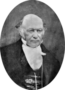 |
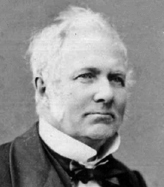
| Giusto Bellavitis | Michail Ostrogradsky | William Hamilton |
The concept of vector, as we know it today, evolved gradually over a period of more than 200 years. The Italian mathematician, senator, and municipal councilor Giusto Bellavitis (1803--1880) abstracted the basic idea in 1835. The idea of an n-dimensional Euclidean space for n > 3 appeared in a work on the divergence theorem by the Russian mathematician Michail Ostrogradsky (1801--1862) in 1836, in the geometrical tracts of Hermann Grassmann (1809--1877) in the early 1840s, and in a brief paper of Arthur Cayley (1821--1895) in 1846. Unfortunately, the first two authors were virtually ignored in their lifetimes. In particular, the work of Grassmann was quite philosophical and extremely difficult to read. The term vector was introduced by the Irish mathematician, astronomer, and mathematical physicist William Rowan Hamilton (1805--1865) as part of a quaternion.
Vectors can be described also algebraically. Historically, the first vectors were Euclidean vectors that can be expanded through standard basic vectors that are used as coordinates. Then any vector can be uniquely represented by a sequence of scalars called coordinates or components. The set of such ordered n-tuples is denoted by \( \mathbb{R}^n . \) When scalars are complex numbers, the set of ordered n-tuples of complex numbers is denoted by \( \mathbb{C}^n . \) Motivated by these two approaches, we present the general definition of vectors.
- Compute u −v and 3u −2v ---> \[ {\bf u} = \begin{bmatrix} -2 \\ \phantom{-}1 \end{bmatrix} , \quad {\bf v} = \begin{bmatrix} 3 \\ 2 \end{bmatrix} \qquad\mbox{and} \qquad {\bf u} = \begin{bmatrix} \phantom{-}1 \\ -1 \end{bmatrix} , \quad {\bf v} = \begin{bmatrix} \phantom{-}4 \\ -3 \end{bmatrix} . \]
-
Write system of equations that is equivalent to the given vector equation.
-
\[ x_1 \begin{bmatrix} \phantom{-}3 \\ -4 \end{bmatrix} + x_2 \begin{bmatrix} -1 \\ -2 \end{bmatrix} + x_3 \begin{bmatrix} \phantom{-}5 \\ -2 \end{bmatrix} = \begin{bmatrix} \phantom{-}1 \\ -1 \end{bmatrix}; \]
-
\[ x_1 \begin{bmatrix} 3 \\ 0 \\ 2 \end{bmatrix} + x_2 \begin{bmatrix} -1 \\ \phantom{-}3 \\ \phantom{-}5 \end{bmatrix} + x_3 \begin{bmatrix} -2 \\ \phantom{-}7 \\ \phantom{-}2 \end{bmatrix} = \begin{bmatrix} 5 \\ 1 \\ 3 \end{bmatrix}; \]
-
\[ x_1 \begin{bmatrix} 2 \\ 1 \\ 7 \end{bmatrix} + x_2 \begin{bmatrix} \phantom{-}3 \\ -2 \\ -5 \end{bmatrix} + x_3 \begin{bmatrix} \phantom{-}4 \\ -6 \\ \phantom{-}1 \end{bmatrix} = \begin{bmatrix} -5 \\ -4 \\ \phantom{-}2 \end{bmatrix} . \]
-
- Given \( \displaystyle {\bf u} = \begin{bmatrix} 2 \\ 1 \\ 3 \end{bmatrix} , \ {\bf v} = \begin{bmatrix} \phantom{-}3 \\ -1 \\ -5 \end{bmatrix} , \quad\mbox{and} \quad {\bf b} = \begin{bmatrix} -5 \\ 5 \\ h \end{bmatrix} . \) For what value of h is b a linear combination of vectors u and v?
- Given \( \displaystyle {\bf u} = \begin{bmatrix} 4 \\ 3 \\ 1 \end{bmatrix} , \ {\bf v} = \begin{bmatrix} \phantom{-}2 \\ -2 \\ -3 \end{bmatrix} , \quad\mbox{and} \quad {\bf b} = \begin{bmatrix} 8 \\ h \\ 9 \end{bmatrix} . \) For what value of h is b a linear combination of vectors u and v?
-
Rewrite the system of equations in a vector form
\[ \begin{split} 2x_1 - 3 x_2 + 7 x_3 &= -1 , \\ -5 x_1 -2 x_2 - 3 x_3 &= 2 , \\ 3x_1 + 2 x_2 + 4 x_3 &= 3 . \end{split} \]
- Let \( \displaystyle {\bf u} = \begin{bmatrix} 3 \\ 1 \end{bmatrix} , \ {\bf v} = \begin{bmatrix} \phantom{-}2 \\ -2 \end{bmatrix} , \quad\mbox{and} \quad {\bf b} = \begin{bmatrix} h \\ k \end{bmatrix} . \) Show that the linear equation x₁u + x₂v = b has a solution for any values of h and k.
-
Mark each statement True or False.
- Another notation for the vector (1, 2) is \( \displaystyle \begin{bmatrix} 1 \\ 2 \end{bmatrix} . \)
- An example of a linear combination of vectors u and v is 2v.
- Any list of of six complex numbers is a vector in ℂ6.
- The vector 2v results when a vector v + u is added to the vector v − u.
- The solution set of the linear system whose augmented matrix is [ a1 a2 a3 b ] is the same as the solution set of the vector equation x₁a₁ + x₂a₂ + x₃a₃ = b.
- Vector addition
- The Mathematical Gazette Vol. 48, No. 363 (Feb., 1964), pp. 34-36 (3 pages). https://doi.org/10.2307/3614306
- Milk