
Introduction to Linear Algebra
Systems of Linear Equations
- Introduction
- Linear systems
- Vectors
- Linear combinations
- Matrices
- Planes in ℝ³
- Equation A x = b
- Sensitivity of solutions
- Linear independence
- Plane transformations
- Space transformations
- Linear transformations
- Affine maps
- Exercises
- Answers
Matrix Algebra
- Introduction
- Manipulation of matrices
- Partitioned matrices
- Block matrices
- Matrix operators
- Determinants
- Cofactors
- Cramer's rule
- Chiò's method
- Equivalent matrices
- Elimination: A = L U
- PLU factorization
- Reflection
- Givens rotation
- Special matrices
- Exercises
- Answers
Vector Spaces
- Introduction
- Motivation
- Vector spaces
- Bases
- Dimension
- Coordinate systems
- Linear transformations
- Change of basis
- Matrix transformations
- Compositions
- Isomorphisms
- Dual transformations
- Quotient spaces
- Rank
- Solving A x = b
- Exercises
- Answers
Eigenvalues, Eigenvectors
- Introduction
- Characteristic polynomials
- Companion matrix
- Algebraic and geometric multiplicities
- Minimal polynomials
- Eigenspaces
- Where are eigenvalues?
- Eigenvalues of A B and B A
- Generalized eigenvectors
- Similarity
- Diagonalizability
- Self-adjoint operators
- Exercises
- Answers
Euclidean Spaces
- Introduction
- Euclidean space
- Bilinear transformations
- Norm and distance
- Matrix norms
- Dual norms
- Dual transformations
- Examples of transformations
- Orthogonality
- Gram--Schmidt Process
- Orthogonal matrices
- Self-adjoint matrices
- Unitary matrices
- Projection operators
- QR-decomposition
- Least Square Approximation
- Quadratic forms
- Exercises
- Answers
Canonical forms
- Introduction
- 2D decomposition
- 3D decomposition
- Projectors
- Direct-sum decompositions
- Cyclic decompositions
- Symmetric matrices
- Pseudoinverse
- URV-decomposition
- LU-decomposition
- QR-decomposition
- Cholesky decomposition
- Schur decomposition
- Positive matrices
- Roots
- Polar factorization
- Spectral decomposition
- CUR decomposition
- Exercises
- Answers
Applications
- Introduction
- Circles along curves
- TNB frames
- GPS problem
- Coriolis acceleration
- Poisson equation
- Graph theory
- Error correcting codes
- Electric circuits
- FSA
- Markov chains
- Cryptography
- Wave-length transfer matrix
- Computer graphics
- Linear Programming
- Hill's determinant
- Fibonacci matrices
- Discrete dynamic systems
- Discrete Fourier transform
- Fast Fourier transform
- Curve fitting
- Answers
Miscellany
- Introduction
- Circles along curves
- TNB frames
- Differential forms
- Calculus
- Vector representations
- Matrix representations
- Change of basis
- Orthonormal Diagonalization
- Generalized inverse
- Differential forms
Preliminaries
- Complex Number Operations
- Sets
- Polynomials
- Polynomials and Matrices
- Computer solves Systems of Linear Equations
- Location of Eigenvalues
- Power Method
- Iterative Method
- Similarity and Diagonalization
Glossary
Reference

This Book is licensed under Creative Commons Attribution-NonCommercial-NoDerivs 3.0 Unported License
Jacobi's scheme
In numerical linear algebra, the Jacobi method (a.k.a. the Jacobi iteration method) is an iterative algorithm for determining the solutions of a strictly diagonally dominant system of linear equations. Each diagonal element is solved for, and an approximate value is plugged in. The method was discovered by Carl Gustav Jacob Jacobi in 1845.
The idea of this iteration method is to extract the main diagonal of the matrix of the given vector equation
Here is the algorithm for Jacobi iteration method:
Input: initial guess x(0) to the solution, (diagonal dominant) matrix A, right-hand side
       vector b, convergence criterion
Output: solution when convergence is reached
Comments: pseudocode based on the element-based formula above

k = 0
while convergence not reached do
    for i := 1 step until n do
        σ = 0
        for j := 1 step until n do
            if j ≠ i then
                σ = σ + aij xj(k)
            end
        end
        xi(k+1) = (bi − σ) / aii
    end
    increment k
end
Jacobi's method begins with solving the first equation for x₁ and the second equation for x₂, to obtain
| n | 0 | 1 | 2 | 3 | 4 | 5 |
|---|---|---|---|---|---|---|
| x₁ | 0 | \( \displaystyle \frac{7}{6} \) | \( \displaystyle \frac{22}{21} \approx 1.04762 \) | \( \displaystyle \frac{101}{63} \approx 1.60317 \) | \( \displaystyle \frac{682}{441} \approx 1.54649 \) | \( \displaystyle \frac{2396}{1323} \approx 1.81104 \) |
| x₂ | 0 | \( \displaystyle -\frac{1}{7} \) | \( \displaystyle \frac{11}{21} \approx 0.52381 \) | \( \displaystyle \frac{67}{147} \approx 0.455782 \) | \( \displaystyle \frac{341}{441} \approx 0.773243 \) | \( \displaystyle \frac{2287}{3087} \approx 0.740849 \) |
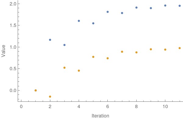
The successive vectors \( \displaystyle \quad \begin{bmatrix} x_1^{(k)} \\ x_2^{(k)} \end{bmatrix} \quad \) are called iterates. For instance, when k = 5, the fifth iterate is \( \displaystyle \quad \begin{bmatrix} 1.8110 \\ 0.740849 \end{bmatrix} \quad \)
Here is Mathematica code to produce the result you see above, first using a module, which is used in other examples also.
In code above, parameter n_ is for the number of iterations you want - the display is always the last 5 iterations; fp_ is for floating point, the default being "True" - if you input "False" as the last argument, you will get an explicit solution, which produces fractions when input coefficients are from ℚ.
jacMeth to our problem.
| Matrix | A | Λ | L | U | b | x0 |
|---|---|---|---|---|---|---|
| \( \displaystyle \begin{pmatrix} 6 & -5 \\ 4 & -7 \end{pmatrix} \) | \( \displaystyle \begin{pmatrix} 6 & 0 \\ 0 & -7 \end{pmatrix} \) | \( \displaystyle \begin{pmatrix} 0&0 \\ 4&0 \end{pmatrix} \) | \( \displaystyle \begin{pmatrix} 0&-5 \\ 0&0 \end{pmatrix} \) | \( \displaystyle \begin{pmatrix} 7 \\ 1 \end{pmatrix} \) | \( \displaystyle \begin{pmatrix} 0 \\ 0 \end{pmatrix} \) | |
| Iterations | 0 | 1 | 2 | 3 | 4 | 5 |
| \( \displaystyle \begin{pmatrix} 0&0 \end{pmatrix} \) | \( \displaystyle \begin{pmatrix} \frac{7}{6} & -\frac{1}{7} \end{pmatrix} \) | \( \displaystyle \begin{pmatrix} \frac{22}{21} & \frac{11}{21} \end{pmatrix} \) | \( \displaystyle \begin{pmatrix} \frac{101}{63} & \frac{67}{147} \end{pmatrix} \) | \( \displaystyle \begin{pmatrix} \frac{682}{441} & \frac{341}{441} \end{pmatrix} \) | \( \displaystyle \begin{pmatrix} \frac{2396}{1323} & \frac{2287}{3087} \end{pmatrix} \) |
Each iteration may be plotted for the separate elements of the solution matrix
Now we repeat calculations by making 50 iterative steps.
N[%]
Expressing the rational numbers above as floating point reals, we get the same result, which is more suitable for human eyes. So, we repeat calculations using floating point representation.
Finally, we can obtain the same result as floating point, also in less than a second.
| Matrix | A | Λ | L | U | b | x0 |
|---|---|---|---|---|---|---|
| \( \displaystyle \begin{pmatrix} 6 & -5 \\ 4 & -7 \end{pmatrix} \) | \( \displaystyle \begin{pmatrix} 6 & 0 \\ 0 & -7 \end{pmatrix} \) | \( \displaystyle \begin{pmatrix} 0&0 \\ 4&0 \end{pmatrix} \) | \( \displaystyle \begin{pmatrix} 0&-5 \\ 0&0 \end{pmatrix} \) | \( \displaystyle \begin{pmatrix} 7 \\ 1 \end{pmatrix} \) | \( \displaystyle \begin{pmatrix} 0 \\ 0 \end{pmatrix} \) | |
| Iterations | 0 | 46 | 47 | 48 | 49 | 50 |
| (2., 1.) | (2., 1.) | (2., 1.) | (2., 1.) | (2., 1.) | (2., 1.) |
Here are the component parts of the code above, producing the same output in steps.
d = DiagonalMatrix[Diagonal[A]];
l = LowerTriangularize[A, -1];
u = UpperTriangularize[A, 1];
b = ({ {7}, {1} });
x[1] = ({ {0}, {0}Sdemo3 });
Grid[{{"A", "d", "l", "u", "b", "x0"}, MatrixForm[#] & /@ {A, d, l, u, b, x[1]}}, Frame -> All]
Starting point does not matter for final destination of Jacobi's ietrating scheme. Let's test that with calculations using different starting points, random floating point numbers and integers. Below, a function is provided that works with a list of starting points.
varSt = MapThread[ Last[Prepend[ FoldList[LinearSolve[d, -(l + u) . # + b] &, {#1, #2}, Range[50]], {"x1", "x2"}]] &,(*starting point->*)stPts][[All, All, 1]];
TableForm[ Transpose[{stPts[[1]], varSt[[All, 1]], stPts[[2]], varSt[[All, 2]]}], TableHeadings -> {None, {"Starting\npoint", "\n\!\(\*SubscriptBox[\(x\), \(1\)]\)", "Starting\npoint", "\n\!\(\*SubscriptBox[\(x\), \(2\)]\)"}}]
| Starting | Starting | ||
|---|---|---|---|
| Point | x₁ | Point | x₂ |
| 0 | 2. | 0 | 1. |
| 0.5 | 2. | 0.5 | 1. |
| 0.25 | 2. | 0.25 | 1. |
| 0.0013514 | 2. | 0.742626 | 1. |
| 10 | 2. | 16 | 1. |
N[Eigenvalues[A]]
| n | 0 | 1 | 2 | 3 | 4 | 5 |
|---|---|---|---|---|---|---|
| x₁ | 0 | \( \displaystyle \frac{4}{5} \) | \( \displaystyle \frac{11}{5} = 2.2 \) | \( \displaystyle \frac{13}{25} = 0.52 \) | \( \displaystyle -\frac{341}{50} = -6.82 \) | \( \displaystyle -\frac{823}{250} = -3.292 \) |
| x₂ | 0 | \( \displaystyle -\frac{5}{2} \) | \( \displaystyle \frac{11}{10} =1.1 \) | \( \displaystyle -\frac{127}{20} = -6.35 \) | \( \displaystyle -\frac{341}{100} = -3.41 \) | \( \displaystyle \frac{2887}{200} = -14.435 \) |
It is hard to believe that this iteration scheme provides the correct answer: x₁ = 2 and x₂ = 1.
b = {4, 10};
LinearSolve[A, b]
Here are the last five runs:
| Matrix | A | Λ | L | U | b | x0 |
|---|---|---|---|---|---|---|
| \( \displaystyle \begin{pmatrix} 5 & -6 \\ 7 & -4 \end{pmatrix} \) | \( \displaystyle \begin{pmatrix} 5 & 0 \\ 0 & -4 \end{pmatrix} \) | \( \displaystyle \begin{pmatrix} 0&0 \\ 7&0 \end{pmatrix} \) | \( \displaystyle \begin{pmatrix} 0&-6 \\ 0&0 \end{pmatrix} \) | \( \displaystyle \begin{pmatrix} 4 \\ 10 \end{pmatrix} \) | \( \displaystyle \begin{pmatrix} 0 \\ 0 \end{pmatrix} \) | |
| Iterations | 48 | 49 | 50 | 51 | 52 | 53 |
| \( \displaystyle \left\{ \begin{array}{c} -1.08216 \times 10^8 , \\ -5.41082 \times 10^7 \end{array} \right\} \) | \( \displaystyle \{ \begin{array}{c} -6.49298 \times 10^7 , \\ -1.89379 \times 10^8 \end{array} \} \) | \( \displaystyle \left\{ \begin{array}{c} -2.27254 \times 10^8 , \\ -3.97695 \times 10^8 \end{array} \right\} \) | \( \displaystyle \{ \begin{array}{c}-4.77234 \times 10^8 , \\ -2.38617 \times 10^8 \end{array} \} \) | \( \displaystyle \left\{ \begin{array}{c} -2.86341 \times 10^8 , \\ -8.3516 \times 10^8 \end{array} \right\} \) | \( \displaystyle \left\{ \begin{array}{c} -2.86341 \times 10^8 , \\ -8.3516 \times 10^8 \end{array} \right\} \) |
To start an iteration method, you need an initial guess vector
|
\begin{equation} \label{EqJacobi.7}
{\bf x}^{(k+1)}_j = \frac{1}{a_{j,j}} \left( b_j - \sum_{i\ne j} a_{j,i} x_i^{(k)} \right) , \qquad j=1,2,\ldots , n.
\end{equation}
|
|---|
If the diagonal elements of matrix A are much larger than the off-diagonal elements, the entries of B should all be small and the Jacobi iteration should converge. We introduce a very important definition that reflects diagonally dominant property of a matrix.
Theorem 2: If a system of n linear equations in n variables has a strictly diagonally dominant coefficient matrix, then it has a unique solution and both the Jacobi and the Gauss--Seidel method converge to it.
b = {5, 21, -9};
LinearSolve[A, b]
However, the code above will not work if you define vector b as column vector. To overcome this, use the following modification.
LinearSolve[A, b][[All,1]]
Upon extracting the diagonal matrix from A, we split the given system (3.1) into the following form: \[ \left( \Lambda + {\bf M} \right) {\bf x} = {\bf b} \qquad \iff \qquad {\bf x} = \Lambda^{-1} {\bf b} - \Lambda^{-1} {\bf M} \,{\bf x} , \] where \[ {\bf d} = \Lambda^{-1} {\bf b} = \begin{bmatrix} \frac{1}{5} & 0 & 0 \\ 0 & \frac{1}{7} & 0 \\ 0 & 0 & \frac{1}{8} \end{bmatrix} \begin{pmatrix} \phantom{-}5 \\ 21 \\ -9 \end{pmatrix} = \begin{bmatrix} 1 \\ 3 \\ - \frac{9}{8} \end{bmatrix} , \qquad {\bf B} = - \Lambda^{-1} {\bf M} = \begin{bmatrix} 0 & \frac{4}{5} & - \frac{1}{5} \\ - \frac{5}{7} & 0 & \frac{4}{7} \\ - \frac{3}{8} & \frac{7}{8} & 0 \end{bmatrix} . \] Matrix B has one real eigenvalue λ₁ ≈ -0.362726, and two complex conjugate eigenvalues λ₂ ≈ 0.181363 + 0.308393j, λ₃ ≈ 0.181363 - 0.308393j, where j is the imaginary unit of the complex plane ℂ, so j² = −1.
Eigenvalues[B]
Although we know exact solution, x₁ = 2, x₂ = 1, x₃ = −1, of the given system of linear equations (3.1), we know that convergence of Jacobi's iteration scheme does not depend on the initial guess. So we start with zero: \[ {\bf x}^{(0)} = \left[ 0, 0, 0 \right] . \]
MatrixForm[%]/
MatrixForm[%]
B= {{0, 4/5, -1/5},{-5/7,0,4/7},{-3/8,7/8,0}};
x2 = d + B.d
B= {{0, 4/5, -1/5},{-5/7,0,4/7},{-3/8,7/8,0}};
x3 = d + B.x2
| Matrix | A | Λ | L | U | b | x0 |
|---|---|---|---|---|---|---|
| \( \displaystyle \begin{pmatrix} 5 & -4 & 1 \\ 5 & 7 & -4 \\ 3 & -7 & 8 \end{pmatrix} \) | \( \displaystyle \begin{pmatrix} 5 & 0& 0 \\ 0 & 7&0 \\ 0&0& 8 \end{pmatrix} \) | \( \displaystyle \begin{pmatrix} 0&0&0 \\ 5&0&0 \\ 3& -7 & 0 \end{pmatrix} \) | \( \displaystyle \begin{pmatrix} 0&-4 & 1 \\ 0&0& -4 \\ 0&0&0 \end{pmatrix} \) | \( \displaystyle \begin{pmatrix} 5 \\ 21 \\ -9 \end{pmatrix} \) | \( \displaystyle \begin{pmatrix} 0 \\ 0 \\ 0 \end{pmatrix} \) | |
| Iterations | 0 | 1 | 2 | 3 | 4 | 5 |
| \( \displaystyle \begin{pmatrix} 0&0&0 \end{pmatrix} \) | \( \displaystyle \begin{pmatrix} 1 & 3 & - \frac{9}{8} \end{pmatrix} \) | \( \displaystyle \begin{pmatrix} \frac{29}{8} & \frac{23}{14} & \frac{9}{8} \end{pmatrix} \) | \( \displaystyle \begin{pmatrix} \frac{117}{56} & \frac{59}{56} & -\frac{67}{64} \end{pmatrix} \) | \( \displaystyle \begin{pmatrix} \frac{4597}{2240} & \frac{713}{784} & -\frac{221}{224} \end{pmatrix} \) | \( \displaystyle \begin{pmatrix} \frac{15091}{7840} & \frac{3043}{3136} & -\frac{2813}{2560} \end{pmatrix} \) |
We repeat calculations with floating point output.
| Matrix | A | Λ | L | U | b | x0 |
|---|---|---|---|---|---|---|
| \( \displaystyle \begin{pmatrix} 5 & -4 & 1 \\ 5 & 7 & -4 \\ 3 & -7 & 8 \end{pmatrix} \) | \( \displaystyle \begin{pmatrix} 5 & 0& 0 \\ 0 & 7&0 \\ 0&0& 8 \end{pmatrix} \) | \( \displaystyle \begin{pmatrix} 0&0&0 \\ 5&0&0 \\ 3& -7 & 0 \end{pmatrix} \) | \( \displaystyle \begin{pmatrix} 0&-4 & 1 \\ 0&0& -4 \\ 0&0&0 \end{pmatrix} \) | \( \displaystyle \begin{pmatrix} 5 \\ 21 \\ -9 \end{pmatrix} \) | \( \displaystyle \begin{pmatrix} 0 \\ 0 \\ 0 \end{pmatrix} \) | |
| Iterations | 0 | 1 | 2 | 3 | 4 | 5 |
| \( \displaystyle \begin{pmatrix} 0&0&0 \end{pmatrix} \) | \( \displaystyle \begin{array}{c} 1. \\ 3. \\ - 1.125 \end{array} \) | \( \displaystyle \begin{array}{c} 3.625, \\ 1.64286, \\ 1.125 \end{array} \) | \( \displaystyle \begin{array}{c} 2.08929, \\ 1.05357, \\ -1.04688 \end{array} \) | \( \displaystyle \begin{array}{c} 2.05223, \\ 0.909439, \\ -0.986607 \end{array} \) | \( \displaystyle \begin{array}{c} 1.92487, \\ 0.970344, \\ -1.09883 \end{array} \) |
We repeat calculations with 20 runs, displaying only the initial and last five:
| Matrix | A | Λ | L | U | b | x0 |
|---|---|---|---|---|---|---|
| \( \displaystyle \begin{pmatrix} 5 & -4 & 1 \\ 5 & 7 & -4 \\ 3 & -7 & 8 \end{pmatrix} \) | \( \displaystyle \begin{pmatrix} 5 & 0& 0 \\ 0 & 7&0 \\ 0&0& 8 \end{pmatrix} \) | \( \displaystyle \begin{pmatrix} 0&0&0 \\ 5&0&0 \\ 3& -7 & 0 \end{pmatrix} \) | \( \displaystyle \begin{pmatrix} 0&-4 & 1 \\ 0&0& -4 \\ 0&0&0 \end{pmatrix} \) | \( \displaystyle \begin{pmatrix} 5 \\ 21 \\ -9 \end{pmatrix} \) | \( \displaystyle \begin{pmatrix} 0 \\ 0 \\ 0 \end{pmatrix} \) | |
| Iterations | 0 | 16 | 17 | 18 | 19 | 20 |
| \( \displaystyle \begin{pmatrix} 0&0&0 \end{pmatrix} \) | (2., 1., −1.) | (2., 1., −1.) | (2., 1., −1.) | (2., 1., −1.) | (2., 1., −1.) |
Theorem 3: If the Jacobi or the Gauss-Seidel method converges for a system of n linear equations in n unknowns, then it must converge to the solution of the system.
Convergence means that "as iterations increase, the values of the iterates get closer and closer to a limiting value:' This means that x(k) converge to r, As usual, we denote by x = c the true solution of the system A x = b.
We must show that r = c. Recall that the Jacobi's (GS is similar) iterates satisfy the equation \[ \Lambda\,{\bf x}^{(k+1)} = {\bf b} + \left( \Lambda - {\bf A} \right) {\bf x}^{(k)} , \qquad k=0,,2,\ldots . \tag{P3.1} \] The Gauss-Seidel method leads to a similar equation where A is further decomposed into upper and lower triangular parts. Application of limit to both sides of Eq.(P3.1), we obtain \[ \Lambda\,{\bf r} = {\bf b} + \left( \Lambda - {\bf A} \right) {\bf r} \qquad \iff \qquad {\bf 0} = {\bf b} - {\bf A}\,{\bf r} . \] Therefore, vector \( \displaystyle {\bf r} = \lim_{k\to \infty} {\bf x}^{(k)} \) satisfies the equation A x = b, so it must be equal to c.
MatrixRank[A]
NullSpace[A]
diag = {{9, 0, 0, 0}, {0, 8, 0, 0}, {0, 0, 7, 0}, {0, 0, 0, 6}};
M = A - diag;
Inverse[diag] . {9, 7, -11, 9}
M = A - diag ;
d = {1, 7/8, -(11/7), 3/2}; B = -Inverse[diag] . M ;
x1 = d + B . d
| n | 0 | 1 | 2 | 3 | 4 | 5 | 10 |
|---|---|---|---|---|---|---|---|
| x₁ | 0 | \( \displaystyle 1 \) | \( \displaystyle \frac{209}{63} \approx 3.31746 \) | \( \displaystyle \frac{40}{189} \approx 0.21164 \) | \( \displaystyle \approx 2.054 \) | \( \displaystyle \approx 2.34034 \) | \( \displaystyle \approx 2.31208 \) |
| x₂ | 0 | \( \displaystyle \frac{7}{8} \) | \( \displaystyle -\frac{89}{112} \approx -0.794643 \) | \( \displaystyle \frac{175}{288} \approx 0.607639 \) | \( \displaystyle \approx 0.305567 \) | \( \displaystyle \approx -0.427675 \) | \( \displaystyle \approx -0.128371 \) |
| x₃ | 0 | \( \displaystyle -\frac{11}{7} \) | \( \displaystyle \frac{1}{2} = 0.5 \) | \( \displaystyle -\frac{1235}{1764} \approx -0.700113 \) | \( \displaystyle \approx -0.922808 \) | \( \displaystyle \approx 0.262426 \) | \( \displaystyle \approx -0.257853 \) |
| x₄ | 0 | \( \displaystyle \frac{3}{2} \) | \( \displaystyle \frac{37}{84} \approx 0.440476 \) | \( \displaystyle \frac{425}{1512} \approx 0.281085 \) | \( \displaystyle \approx 1.25112 \) | \( \displaystyle \approx 0.250038 \) | \( \displaystyle \approx 0.729597 \) |
We are going to make a numerical experiment and check whether Jacobi's iteration depends on the initial guess, which we take closer to the true values: x(0) = [1.5, 0.5, 2.5, 3.5]. Using iteration (4.3), we calculate Jacobi's approximants.
| n | 0 | 1 | 2 | 3 | 4 | 5 | 10 |
|---|---|---|---|---|---|---|---|
| x₁ | 1.5 | 1.61111 | 2.16138 | 1.84245 | 1.84634 | 2.09821 | 1.99034 |
| x₂ | 0.5 | 0.9375 | 0.731647 | 0.810433 | 0.906534 | 0.738926 | 0.815846 |
| x₃ | 2.5 | 2.14286 | 2.35317 | 2.355912.35591 | 2.18519 | 2.37932 | 2.2872 |
| x₄ | 3.5 | 3.41667 | 3.37368 | 3.22828 | 3.3894 | 3.3099 | 3.35227 |
Mathematica confirms these calculations.
This table of iterative values shows that the first coordinate plays around true value x₁ = 2, but we cannot claim convergence of other coordinates, except probably x₂ = 1.
| Matrix | A | Λ | L | U | b | x0 |
|---|---|---|---|---|---|---|
| \( \displaystyle \begin{pmatrix} 9 & -8 & 5&4 \\ 1 & 8 & -5&3 \\ =2 & -4 & 7&-6 \\ 2&-4&-5&6 \end{pmatrix} \) | \( \displaystyle \begin{pmatrix} 9 & 0& 0&0 \\ 0 & 8&0&0 \\ 0&0& 7&0 \\ 0&0&0&6 \end{pmatrix} \) | \( \displaystyle \begin{pmatrix} 0 & 0 & 0&0 \\ 1 & 0 & 0&0 \\ =2 & -4 & 0&0 \\ 2&-4&-5&0 \end{pmatrix} \) | \( \displaystyle \begin{pmatrix} 0 & -8 & 5&4 \\ 0 & 0 & -5&3 \\ 0 & 0 & 0&-6 \\ 0&0&0&0 \end{pmatrix} \) | \( \displaystyle \begin{pmatrix} 9 \\ 7 \\ -11 \\ 9 \end{pmatrix} \) | \( \displaystyle \begin{pmatrix} 0 \\ 0 \\ 0 \\ 0\end{pmatrix} \) | |
| Iterations | 0 | 46 | 47 | 48 | 49 | 50 |
| (0, 0, 0, 0) | {1.67103, 0.131896, -0.455655, 0.651516} |
{1.65994, 0.137018, -0.46018, 0.651207} |
{1.66687, 0.135692, -0.460686, 0.654547} |
{1.66746, 0.133257, -0.4566, 0.650932} |
{1.66142, 0.137093, -0.460923, 0.652518} |
Input: square matrix A and vector b
n is the size of A and vector b
    whle precision condition  do
       for i=1 : n do
           s=0
	   for j=1 : n do
	       if j ≠ i then
	   s = s + 𝑎i,jxj
	       endif
	   endfor
	   yi = (bi−s)/𝑎i,i
	endfor
	   x=y
endwhile
- Anton, Howard (2005), Elementary Linear Algebra (Applications Version) (9th ed.), Wiley International
- Beezer, R., A First Course in Linear Algebra, 2015.
- Beezer, R., A Second Course in Linear Algebra, 2013.