The Wolfram Mathematica notebook which contains the code that produces all the Mathematica output in this web page may be downloaded at this link.
Caution: This notebook will evaluate, cell-by-cell, sequentially, from top to bottom. However, due to re-use of variable names in later evaluations, once subsequent code is evaluated prior code may not render properly. Returning to and re-evaluating the first Clear[ ] expression above the expression no longer working and evaluating from that point through to the expression solves this problem.
$Post :=
If[MatrixQ[#1],
MatrixForm[#1], #1] & (* outputs matricies in MatrixForm*)
Remove[ "Global`*"] // Quiet (* remove all variables *)
Recall that 𝔽 denotes one of the following fields of numbers: ℤ, integers, ℚ, rational numbers, ℝ, real numbers; hence we exclude from our consideration ℂ, complex numbers in this section. It is caused by applications of affine transformations in geometry and computer graphics that utilize only real numbers. We denote by 𝔽m×n or 𝔽m,n the vector space of m-by-n matrices with entries from field 𝔽.
According to Wikipedia, the term linear function can refer to two distinct concepts, based on the context:
In Calculus, a linear function is a polynomial function of degree zero or one; in other words, a function of the form f(x) = m x + b for some constants m and b ∈ ℝ.
In Linear Algebra, a linear function is a linear mapping, or linear transformation: f(λx + y) = λf(x) + f(y). for any scalar λ and any two vectors x and y.
A matrix A of size m-by-n (written as m x n) defines a linear map upon multiplication from left:
Such a map has the basic property A 0 = 0 for column vectors and 0 A = 0 for row vectors.
$Post :=
If[MatrixQ[#1],
MatrixForm[#1], #1] & (* outputs matrices in MatrixForm*)
Remove[ "Global`*"] // Quiet (* remove all variables *)
Affine Transformations
An affine transformation or affinity (in 1748, Leonhard Euler introduced the term affine, which stems from the Latin, affinis, "connected with") is a geometric transformation that preserves the parallelism of lines and the ratio of distances between points.
Affine transformation is closely related to projective transformation---this technique is widely used in computer graphics, image processing, machine learning, and neural networks to perform geometric transformations in a
simple way using transformation matrices.
Although there are several open computer vision libraries for affine transformations such as openGL and
openCV, we prefer to use Mathematica and its build-in commands: AffineTransform and TransformationMatrix.
The following definition may give an impression that an affine transformation is not a general object as it is expected in mathematical literature---formal/abstract definition will be given later. However, it provides us an idea where affine transformations come from. Also, it can be shown (see, for instance, Kostrikin & Manin's book) that any affine transformation is isomorphic to the following algebraic approach.
(Algebraic Representation)
Any map f : 𝔽n×1 ↣ 𝔽m×1
of the form
\begin{equation} \label{EqAffine.1}
\mathbb{F}^{n\times 1} \ni \mathbf{x} \longrightarrow f({\bf x}) = {\bf A}\,{\bf x} + \mathbf{b}
\end{equation}
for some fixed column vector b ∈ 𝔽m×1 and m-by-n matrix A, is called an affine map or transformation. Similarly, a mapping between row vectors
\begin{equation} \label{EqAffine.2}
\mathbb{F}^{1\times m} \ni \mathbf{v} \longrightarrow f({\bf v}) = {\bf v}\,{\bf A} + \mathbf{w}
\end{equation}
for some given row vector w ∈ 𝔽1×n, is also called an affine transformation.
Both formulae \eqref{EqAffine.1} and \eqref{EqAffine.2} are just short cuts of the general transformation of the form (system of linear equations)
Affine map is a geometric transformation that preserves co-linearity (i.e., all points lying on a line initially still lie on a line after
transformation) and ratios of distances (e.g., the
midpoint of a line segment remains the midpoint
after transformation), but not necessarily Euclidean distances and angles.
Since f(0) = b, such a map can be
be linear only when b = 0 in Eq.\eqref{EqAffine.1} or w = 0 in Eq.\eqref{EqAffine.2}. Formulae \eqref{EqAffine.1} and \eqref{EqAffine.2} show that an affine transformation is the composition of a linear transformation (including scaling, homothety, similarity, reflection, rotation, shearing) and a translation.
Example 1:
There are a few countries (exclusively by the U.S. and its formerly and presently governed territories, in addition to a few South American and some countries in the Pacific) that still use Fahrenheit (°F) temperature scale while the majority of countries utilize the International System of Units (SI), which includes Celsius (°C) scale. First proposed in 1724 by physicist Daniel Gabriel Fahrenheit (who had also invented the mercury thermometer in 1714), the Fahrenheit temperature scale was used before domination of metric unit system. Celsius scale is named after the Swedish astronomer Anders Celsius (1701–1744), who developed a variant of it in 1742.
Today, however, Fahrenheit has been replaced by the Celsius (and in scientific applications, Kelvin) scale in all but a handful of the world's countries.
On the kelvin scale, 0°K is equal to −273.15 °C and the boiling point of water is 373°K, which is 100°C.
\[
\mbox{F}^{\circ} = \frac{9}{5}\,\mbox{C}^{\circ} + 32 .
\]
For converting Fahrenheit (°F) into Celsius (°C) scale, use the formula:
\[
\mbox{C}^{\circ} = \frac{5}{9} \left( \mbox{F}^{\circ} - 32^{\circ} \right) .
\]
Note that both, the transformation from Fahrenheit scale into Celsius scale and its reverse, are not linear maps because they do not preserve zero. Actually, these transformations are affine ones.
■
End of Example 1
Basically, there are five affine transformations or their compositions in 2D and 3D:
Translate moves a set of points a fixed distance in each coordinate.
Scale scales a set of points up or down in each coordinate.
(Proper) Rotation (with determinant +1) rotates a set of points about the origin in counterclockwise direction,
Shear offsets a set of points a distance proportional to their x, y or/and z coordinates.
Note that only shear and non-uniform scale change the shape determined by a set of points. A subclass of affine transformations that locally preserves angles, but not necessarily lengths is called the set of conformal maps.
Example 2:
Let us consider an affine transformation
\[
\begin{split}
x &\mapsto x+y +1 , \\
y &\mapsto 2\,y - 1 .
\end{split}
\]
It is convenient to rewrite this transformation in matrix/vector form using either column vectors
\[
\begin{bmatrix} x \\ y \end{bmatrix} \,\mapsto \, \begin{bmatrix} 1 & 1 \\ 0 & 2 \end{bmatrix} \begin{bmatrix} x \\ y \end{bmatrix} + \begin{bmatrix} \phantom{-}1 \\ -1 \end{bmatrix}
\]
or row vectors
\[
\begin{bmatrix} x & y \end{bmatrix} \,\mapsto \, \begin{bmatrix} x & y \end{bmatrix} \begin{pmatrix} 1&0 \\ 1&2 \end{pmatrix} +
\begin{bmatrix} 1 & -1 \end{bmatrix} .
\]
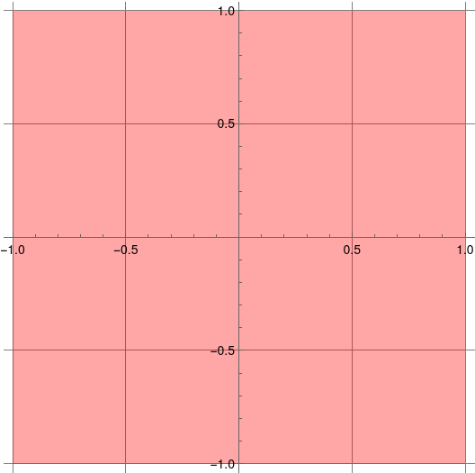
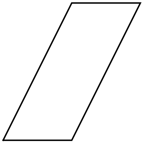
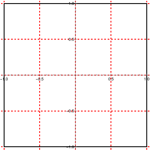
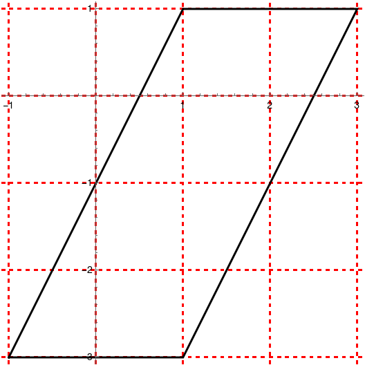
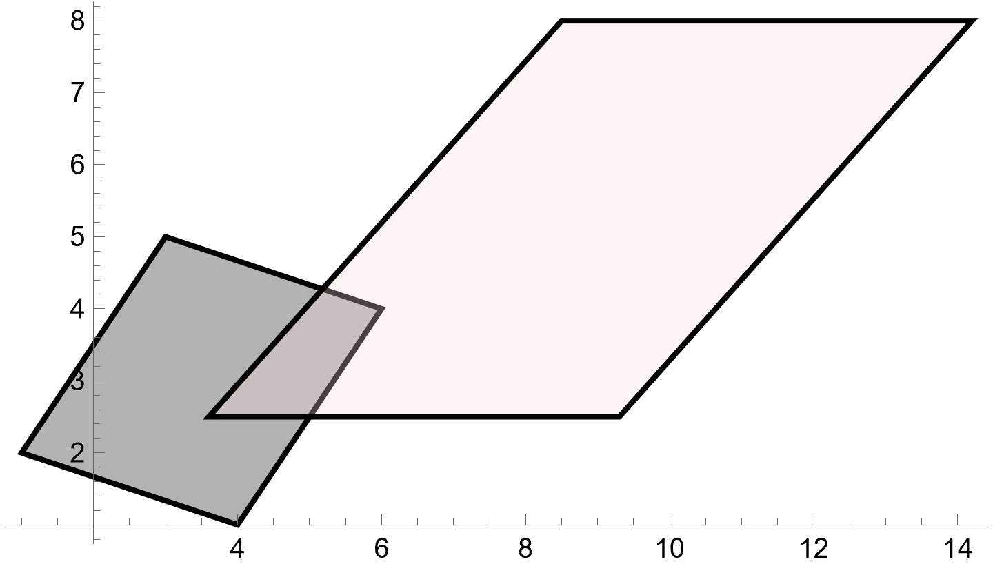
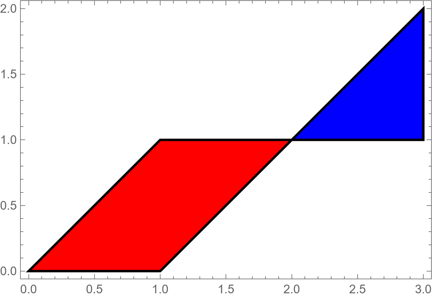
It is a “shear” followed by a translation. The
effect of this shear on the square (𝑎, b, c, d) is shown in the following figure. The
image of this square is the parallelogram.
Then vertical line x = −1 is mapped into the line
\[
x \mapsto y , \qquad y \mapsto 2\,y - 1 .
\]
The images of vertices become
\[
\left( -1,-1 \right) \mapsto \left( -1, -3 \right) , \quad \left( -1, 1 \right) \mapsto \left( 1, 1 \right) , \quad \left( 1, 1 \right) \mapsto \left( 3, 1 \right) , \quad \left( 1, -1 \right) \mapsto \left( 1, -3 \right) .
\]
Since Wolfram has a documentation for AffineTransform, we are going to use its command Affine Transform[m,b].
Note that we are using the second version of the AffineTransform. It has an argument set which is a list, {m, v}, where m is a linear transform and v is a shift (translate) vector. Note below the TransformationFunction it produces is an augmented matrix in the usual form with the b vector the far right column to the right of the dividing line.
The lower left coordinate of our rectangle to be transformed is {-1,-1}. We can use our AffineTransform as function, t, and apply that to the lower left coordinate to get the image of that coordinate.
The transformation function performs two operations: The linear transformation associated with the "m" matrix is the first. The second is the translation association with the "b" vector.
Applying the transform to each corner of the rectangle, we get the same transformed vertices images as provided in the narration above
Wolfram has a function, FindGeometricTransform, which essentially reverses the process we just completed. Below we provide Mathematica with just the new corners, the original corners and ask for an Affine Transform matrix. It returns our matrix above.
One might reasonably ask: "What does the last line mean? What does the row containing {0.,0.|1.}, of the TransformationFunction do?" Those questions come after answering the broader question: "What makes a mathematician?" Getting close to these answers takes a little thought about the order of learning things. A mathematician might say the first questions are premature. We will answer them later in this lesson, further down the page you are reading. But people today are impatient. Wolfram Mathematica version 14 offers a "Chat-Enabled Notebook" with a direct "tap" on the wonders of Artificial Intelligence. You can ask one of many Large Language Models your questions about that last line of the Transformation Function. Here is the answer you might get:
The last row "0 0 1" of a 3x3 transformation matrix is a part of the homogeneous coordinate representation used in affine transformations.
In homogeneous coordinates, a 2D point (x, y) is represented as (x, y, 1) and a 2D vector is represented as (x, y, 0). The reason for this is to allow for translations to be represented as matrix multiplications.
The "0 0 1" row in the transformation matrix ensures that when this matrix is multiplied with a point represented in homogeneous coordinates, the 1 in the third component of the point stays a 1. This is necessary to keep the point a point, and not a vector.
In contrast, if the transformation matrix is multiplied with a vector, the 0 in the third component of the vector stays a 0, ensuring that the vector remains a vector and is not translated.
So, the "0 0 1" row is essentially a part of the mathematical machinery that allows for points and vectors to be treated differently by affine transformations, particularly translations. It doesn't directly affect the scaling, rotation, shear or translation applied to the points or vectors.
For now, patience is advised as we will revisit this later, in subsection devoted to augmented (affine) matrices.
■
End of Example 2
Theorem 1:
If an affine transformation has an inverse, then it is also an affine
transformation.
Let q = A x + b be an affine transformation written for column vectors. It has an inverse only when A is nonsingular matrix, so det(A) ≠ 0. Then A x = q − b. Application of inverse matrix (which exists for nonsingular matrices) to the latter, we obtain x = A−1q − A−1b. `Hence, x = B q + v, where B = A−1 and v = − A−1b.
Example 3:
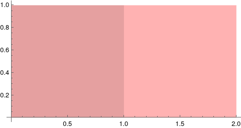
Matrix \( \displaystyle \quad \mathbf{A} = \begin{bmatrix} 1 & 0 \\ 0&0 \end{bmatrix} \) maps all points to the x-axis, so
it is a projection on this axis. The area of any closed
region will become zero. We have det(A) = 0, which verifies that any closed
region’s area will be scaled by zero.
In general, for any given closed region, the area under an affine transformation A x + b is scaled by det(A). This result is valid for any linear mapping y = A x.
Illustrating this in Mathematica requires some careful definitions and distinguishing a transformation matrix with a zero determinant from one with a non-zero determinant. First, we define a transformation matrix, A, which has a zero determinant
This transformation matrix collapses the square into a line, which makes it impossible for Mathematica's Area function to compute the area since a line has no area.
Now we use a transformation matrix, B, with a non-zero determinant.
The basic properties of affine transformations are summarized in the following statement.
Theorem 2:
Let f(x) = A x + b be an affine transformation. Then f
maps a line to a line,
maps a line segment to a line segment,
preserves the property of parallelism among lines and line segments
maps an n-gon to an n-gon,
maps a parallelogram to a parallelogram,
preserves the ratio of lengths of two parallel segments, and
preserves the ratio of areas of two figures.
Let L be a line and let L: p + tm, t ∈ ℝ, be an equation of L in vector form. Then for every t ∈ ℝ,
\[
f \left( \mathbf{p} + t\,{\bf m} \right) = \mathbf{A}\left( \mathbf{p} + t\,{\bf m} \right) + \mathbf{b} = \mathbf{p}_1 + t\,\mathbf{m}_1 ,
\]
where p₁ = A p + b and m₁ = A m. Hence, f(L) = L₁, where L₁ : p₁ + tm₁, t ∈ ℝ, is again a line.
The proof is the same as that for (1), with t restricted to [0, 1].
Suppose that L: p + tm and L₁ : p₁ + tm₁, t ∈ ℝ, are parallel lines. Then m₁ = km for some k ∈ ℝ. Therefore,
\begin{align*}
f \left( \mathbf{p} + t\,\mathbf{m} \right) &= \mathbf{A} \left( \mathbf{p} + t\,\mathbf{m} \right) + {\bf b} = \left( \mathbf{A}\,\mathbf{p} + {\bf b} \right) + t \left( {\bf A}\,{\bf m} \right) = \mathbf{q} + t\,\mathbf{n} ,
\\
f \left( \mathbf{p}_1 + t\,\mathbf{m}_1 \right) &= f \left( \mathbf{p}_1 + t\,k\,\mathbf{m} \right) =
\mathbf{A} \left( \mathbf{p}_1 + t\,k\,\mathbf{m} \right) + {\bf b}
\\
&= \left( \mathbf{A} \, \mathbf{p}_1 + {\bf b} \right) + t \left( \mathbf{A} \,k\,{\bf m} \right) = \mathbf{p}_2 + t\,\mathbf{m}_2 .
\end{align*}
That is, L and L₁ are mapped to lines that are parallel.
It is clear that for two line segments or a line and a line segment the proof is absolutely
analogous.
We prove this by strong induction on n. For the base case, when n = 3, consider a triangle T.
Then T and its interior can be represented in vector form as T :
u + sv + tw, where s, t ∈ [0, 1],
s + t ≤ 1, and the vectors v and w are not collinear. Then
\begin{align*}
f(T) &= F \left( {\bf u} + s {\bf v} + t {\bf w} \right) = \mathbf{A} \left( {\bf u} + s {\bf v} + t {\bf w} \right) + {\bf b}
\\
&= \left( {\bf A}\,{\bf u} + {\bf b} \right) + s \left( \mathbf{A}\,{\bf v} \right) + t \left( \mathbf{A}\,{\bf w} \right)
\\
&= {\bf u}_1 + s{\bf v}_1 + t{\bf w}_1 ,
\end{align*}
where s, t ∈ [0, 1], s + t ≤ 1. By part3, v₁ = Av and w₁ = Aw are not parallel. Thus, T is mapped
to a triangle T₁, which completes the proof of the base case.
Now suppose that f maps each n-gon to an n-gon for all n, 3 ≤ n ≤ k, and let P be a
polygon with k + 1 sides. We know that every polygon with
at least 4 sides has a diagonal contained completely in its interior. Let
\( \displaystyle \quad \overline{AB} \) be such a diagonal
in P. This diagonal divides P into two polygons, P₁ and P₂ containing t and k + 1 − t sides,
respectively, for some t, 3 ≤ t ≤ k. By the inductive hypothesis, f(P₁) and f(P₂) will be
t-sided and (k + 3 − t)-sided polygons, respectively. Since each of these polygons will have
the segment from f(A) to f(B) as a diagonal, the union of P₁ and P₂ will form a polygon with k + 1 sides, which concludes the proof.
The proof that a parallelogram is mapped to a parallelogram is analogous to the proof
that triangles get mapped to triangles in part (4), by simply dropping the condition that s + t ≤ 1.
Consider parallel line segments, S₁ and S₂, given in vector form as Si : pi + tui, t ∈ [0, 1].
Because they are parallel, u₂ = ku₁ for some k ∈ ℝ. As |ui| is the length of Si , the ratio of
lengths of S₂ and S₁ is |k|. From parts (1) and (2), Si is mapped into a segment of length |Aui|. Since Au₂ = A(ku₁) = k(A u), |Au₂| = |k| |Au₁|, which shows that the ratio of lengths
of f(S₂) and f(S₁) is also |k|.
You are encouraged to prove this property!
Example 5:
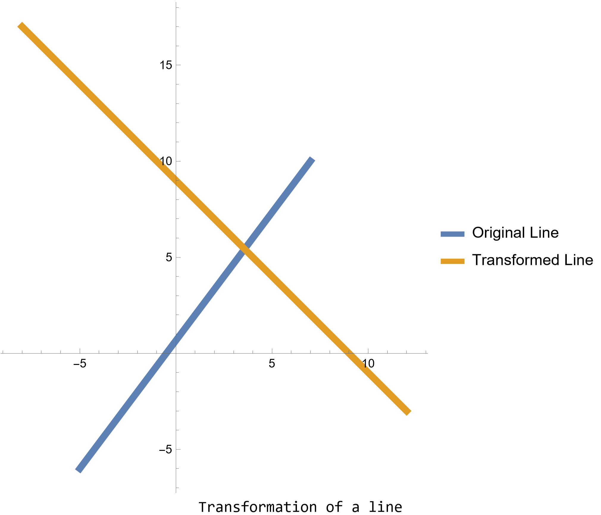
Part 1:
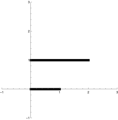
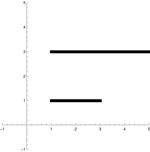
In order to illustrate the first property, we plot a line and compare it with transformed line. For this specific example, the transformation is a translation by the vector b, so the transformed line will be parallel to the original line and offset by the vector b. We consider Eq.(1) when
\[
{\bf A} = \begin{bmatrix} 1&-2 \\ 3&-1 \end{bmatrix} , \qquad {\bf b} = \begin{bmatrix} 5 \\ 6 \end{bmatrix} .
\]
Clear[p, m, A, b, p1, m1];
p = {1, 2};
m = {3, 4};
A = {{1, -2}, {3, -1}};
b = {5, 6};
p1 = A . p + b;
m1 = A . m;
Labeled[
ParametricPlot[{p + t*m, p1 + t*m1}, {t, -2, 2},
PlotStyle -> Thickness[0.016],
PlotLegends -> {"Original Line",
"Transformed Line"}], "Transformation of a line"]
Transformation of a line.
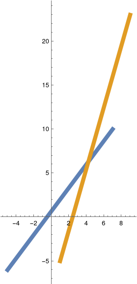
Part 2:
We consider affine transformation
\[
\begin{bmatrix} x \\ y \end{bmatrix} \,\to\, \begin{bmatrix} 2&-1 \\ 1&1 \end{bmatrix} \begin{bmatrix} x \\ y \end{bmatrix} + \begin{bmatrix} 5 \\ 6 \end{bmatrix} .
\]
Generated plot shows that this transformation maps lines into lines.
Using Mathematica, we define the affine transformation and then plot the original straight line and its output.
Clear[p, m, A, b, p1, m1];
p = {1, 2};
m = {3, 4};
A = {{2, -1}, {1, 1}};
b = {5, 6};
p1 = A . p + b;
m1 = A . m;
Labeled[ParametricPlot[{p + t*m, p1 + t*m1}, {t, -2, 2},
PlotStyle -> Thickness[0.03],
PlotLegends -> {"Original Line",
"Transformed Line"}], "Transformation of a line segment"]
Transformation of a line segment.
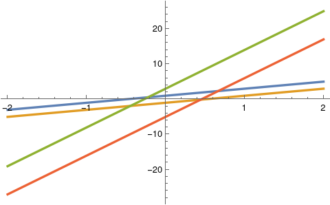
Part 3:
We generate a plot showing the original lines and their transformed versions. The transformed lines are parallel to each other, just like the original lines. First, we define the affine transformation
Part 4:
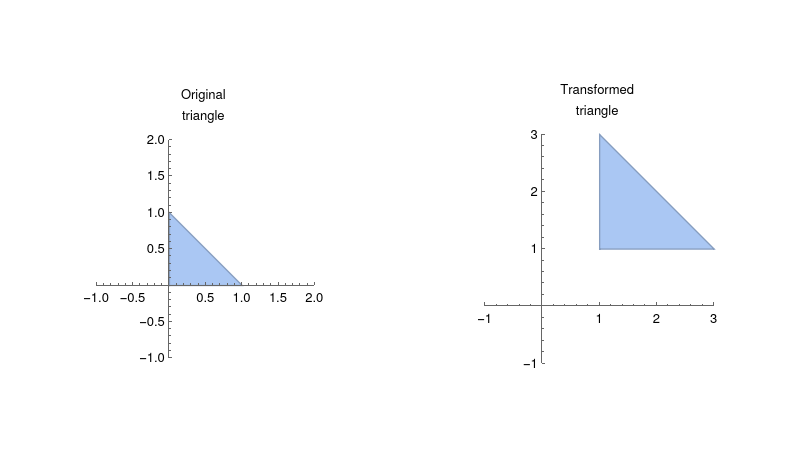
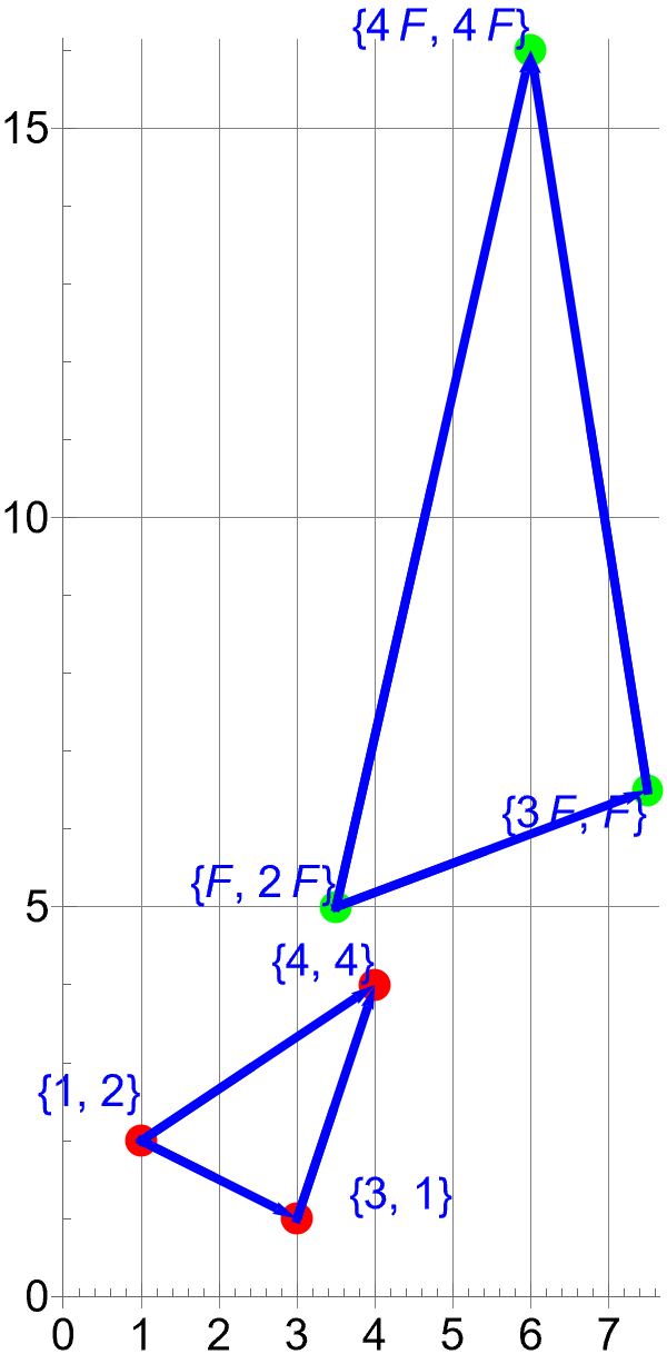
We have two parts. The first part plots a triangle T and its transformed triangle T1 side by side. T is mapped to T1 by the affine transformation.
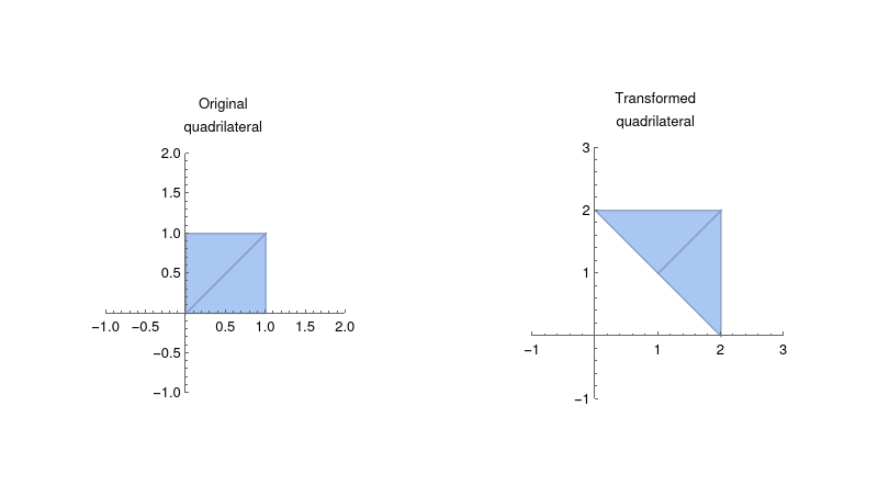
The second part of item #4 generalized further by plotting an original quadrilateral (as two triangles) and the transformed quadrilateral (also as two triangles, which is no longer a quadrilateral). The original is mapped to the transformed one by the affine transformation.
Here we need to illustrate that an affine transformation preserves the ratio of lengths. We can do this by defining a line segment and its transformation, then verifying the ratio of lengths before and after the transformation.
Let's consider a simple affine transformation f(x) = A x + b with
\[
{\bf A} = \begin{bmatrix} 3&4 \\ -1&2 \end{bmatrix} , \qquad {\bf b} = \begin{bmatrix} 2 \\ -1 \end{bmatrix} ,
\]
and four line segments
S₃ = [1,2] of length √5 and S₂ = [2, 4], S₃ = [4, 2], S₄ = [−2, 4] of length √20, which is twice the length of S₁.
After transformation, these will become f(S₁) = [13, 2] and f(S₂) = [24, 5], f(S₃) = [22, 1], f(S₄) = [12, 9].
A = {{3, 4}, {-1, 2}}; b = {{2}, {-1}};
A . {1, 2} + b
{{13}, {2}}
A . {2, 4} + b
{{24}, {5}}
A . {4, 2} + b
{{22}, {-1}}
A . {-2, 4} + b
{{12}, {9}}
Now we calculate the ratios of lengths of transformed segments (with the aid of Mathematica)
N[Norm[A . {2, 4} + b]/Norm[A . {1, 2} + b]]
1.86386
and
N[Norm[A . {4, 2} + b]/Norm[A . {1, 2} + b]]
1.67436
N[Norm[A . {-2, 4} + b]/Norm[A . {1, 2} + b]]
1.14043
None of these ratios is 2, as you expect. Now we answer why these ratios are different. When vector v [1, 2] is subject to affine transformation, its lenth is ∥A v∥ independently of shift vector b, but not ∥A v + b∥ because shift by any vector (b in our case) does not change its length. Therefore, the lengths of affine transformation f(v) are
\begin{align*}
\| f(S_1 ) \| &= \| {\bf A}\,[1, 2] \| = \| [11, 3] \| = \sqrt{130} ,
\\
\| f(S_2 ) \| &= \| {\bf A}\,[2, 4] \| = \| [22, 6] \| = 2\,\sqrt{130} ,
\\
\| f(S_3 ) \| &= \| {\bf A}\,[4, 2] \| = \| [20, 0] \| = 20 ,
\\
\| f(S_4 ) \| &= \| {\bf A}\,[-2, 4] \| = \| [10, 10] \| = 10\,\sqrt{2} .
\end{align*}
Norm[A . {1, 2}]
Sqrt[130]
Norm[A . {2, 4}]
2 Sqrt[130]
On the other hand,
Norm[A . {4, 2}]
20
Norm[A . {-2, 4}]
10 Sqrt[2]
We plot the original line segments S₁ and S₂ and the transformed line segments f(S₁) and f(S₂). The ratio of the lengths of the transformed line segments is 2, which is the same as the ratio of the lengths of the original line segments.
Define an affine transformation x ↦ A x + b, where
\[
{\bf A} = \begin{bmatrix} -3&2 \\ \phantom{-}1&2 \end{bmatrix} , \qquad {\bf b} = \begin{bmatrix} \phantom{-}2 \\ -4 \end{bmatrix} .
\tag{5.7.1}
\]
We apply a build-in command AffineTransform.
It is the subroutine that takes two inputs, m and b and outputs an affine transformation function (which we name "t" in the following code).
m = {{-3, 2}, {1, 2}}
b = {2, -4};
t = AffineTransform[{m, b}]
Apply the transformation to the polygons. We first determine equations of lines that enclose the parallelogram. For example, the line y = 0 is transferred according to affine transformation
\[
\begin{split}
X &= -3\,x + 2\,y +2 , \\
Y &= x + 2\,y -4
\end{split}
\]
leads to the pair
\[
\begin{split}
X &= -3\,x +2 , \\
Y &= x -4 .
\end{split}
\]
From the latter, we get x = Y + 4. Substitution of x into the former equation, we obtain
\[
X = -3 \left( Y+4 \right) +2 \qquad \Longrightarrow \qquad X = -3\,Y + 10 .
\]
Similarly, we express in new coordinates the equation of lines that embrace the given parallelogram:
\begin{align*}
y = 0 \ & \mapsto \ Y = -\frac{1}{3}\,X - \frac{10}{3} ,
\\
y = x \ & \mapsto \ Y = -3\,X + 2 ,
\\
y = 1 \ & \mapsto \ Y = - \frac{1}{3}\, X - \frac{2}{3} ,
\\
y = x -1 \ & \mapsto \ Y = -3\,X + 6 .
\end{align*}
So the corresponding vertices are mapped as follows:
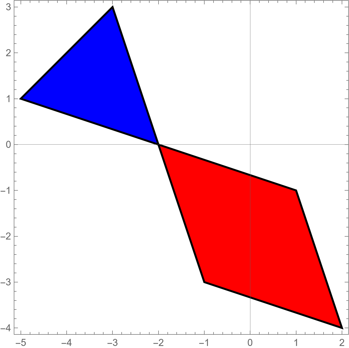
legEG5g = Labeled[GraphicsRow[
{
Graphics[{Red, parallelogram, Blue, triangle}, Frame -> True,
Axes -> True],
Graphics[{Red, transformedParallelogram, Blue,
transformedTriangle}, Frame -> True, Axes -> True]
},
ImageSize -> Large
], "Transformed graphics with equal ratio of area"]
(* Print the result *)
Print["Ratio before transformation: ", ratioBefore];
Print["Ratio after transformation: ", ratioAfter];
Print["Are the ratios equal? ", ratiosEqual];
Parallelogram and triangle.
Areas after affine map.
Part 7A:
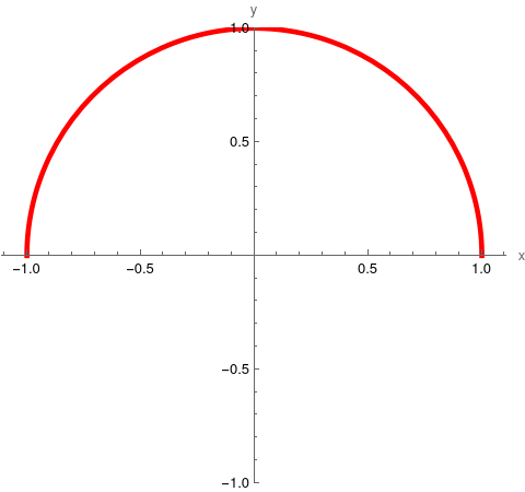
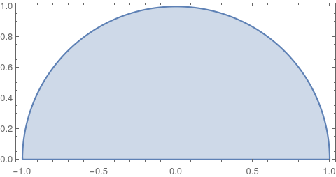
Now we extend this part by considering a half unit circle instead of triangle:
\[
C = \left\{ (x, y) \in \mathbb{R}^2 \ : \ 0 \le x^2 + y^2 \le 1, \quad x\ge 0, \ y\ge 0 \right\} .
\tag{5.7.2}\]
is 1, the ratio of areas of semi-circle to the parallelogram becomes
\[
\frac{\mbox{area of semicircle}}{\mbox{area of parallelogram}} = \frac{\pi /2}{1} = \frac{\pi}{2} = \approx 1.5708 .
\]
N[Pi/2]
1.5708
The equation of the upper boundary of the given semi-circle is
\[
\partial C := \sqrt{1 - x^2} = y , \qquad x\ge 0, \ y\ge 0 .
\]
In order to determine the equations of the boundary of the transformed region, we invoke the affine transformation:
\[
\begin{split}
X &\mapsto \ -3\,x + 2\,y +2 , \\
Y &\mapsto \ x + 2\,y -4
\end{split}
\]
because the affine transformation is given in matrix/vector form:
\[
\begin{bmatrix} X \\ Y \end{bmatrix} = \begin{bmatrix} -3&2 \\ \phantom{-}1 & 2\end{bmatrix} \begin{bmatrix} x \\ y \end{bmatrix} + \begin{bmatrix} \phantom{-}2 \\ -4 \end{bmatrix} .
\]
We can express old variables (x, y) through new ones (X, Y):
\begin{align*}
x &= \frac{1}{4} \left( 6 - X + Y \right) ,
\\
y &= \frac{1}{8} \left( 10 + X + 3\, Y \right) .
\end{align*}
Solve[{X == -3*x + 2*y + 2, Y == x + 2*y - 4}, {x, y}]
{{x -> 1/4 (6 - X + Y), y -> 1/8 (10 + X + 3 Y)}}
We can express this inverse transformation in succinct form:
\[
\begin{bmatrix} x \\ y \end{bmatrix} = \frac{1}{8} \begin{bmatrix} -2&2 \\ \phantom{-}1 &3 \end{bmatrix} \begin{bmatrix} X \\ Y \end{bmatrix} + \begin{bmatrix} 3/2 \\ 5/4 \end{bmatrix}
\tag{5.7.3}
\]
because
\[
{\bf A}^{-1} = \frac{1}{8} \begin{bmatrix} -2&2 \\ \phantom{-}1 & 3 \end{bmatrix} , \qquad \det{\bf A} = -8 .
\]
Inverse[{{-3, 2}, {1, 2}}]
{{-(1/4), 1/4}, {1/8, 3/8}}
Since the boundary of the semicircle consists of two pieces
\begin{align*}
y &= \sqrt{1 - x^2} , \quad -1 \le x \le 1,
\\
y &= 0 , \quad -1 \le x \le 1,
\end{align*}
we need to determine equations of these two pieces in new variables. The equation of straight line y = 0 was determined previously (as a part of parallelogram's boundary):
\[
Y = - \frac{1}{3} \left( X-2 \right) -4 , \qquad 5 \ge X \ge -1 .
\tag{5.7.4}
\]
Note that the new variable X moves in opposite direction because determinant of matrix A is negative. Equation (5.7.4) follows from affine transformations of endpoints:
\begin{align*}
(1, 0) &\mapsto\ (-1, -3) , \\
(-1,0) &\mapsto\ (5, -5) .
\end{align*}
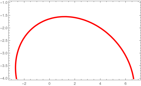
Now we determine the equation of transformed semi-circle. We substitute into the equation of semi-circle
\( \displaystyle \quad x^2 + y^2 = 1 , \quad y \ge 0 . \)
instead of old variables (x, y) their expressions from Eq.(5.7.3) to obtain
\[
2 \left( 6 -X + Y \right)^2 + \left( 10 + X + 3\,Y \right)^2 = 8^2 , \qquad 5 \ge X \ge -1, \quad -4 \le Y \le -2 .
\tag{5.7.5}
\]
The alert student might compare the range of X and the range of Y above with the ranges of the code for the same variables immediately below. While they are different, it is of no matter as using a different ranges in the code just changes the perimeter white space in the graphic.
Labeled[ContourPlot[
2*(6 - X + Y)^2 + (10 + X + 3*Y)^2 == 8^2, {X, -3, 7}, {Y, -4, -1},
ContourStyle -> {Red, Thickness[0.01]},
AspectRatio ->
0.6], "Transformed upper Boundary\nof a unit semi circle"]
Transformed upper Boundary of a unit semi-circle.
The figure above does not provide a true presentation because Mathematica plots it using standard ordering of independent variable. You need to flip it with respect to ordinate (vertical axis) to obtain a true picture.
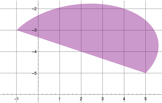
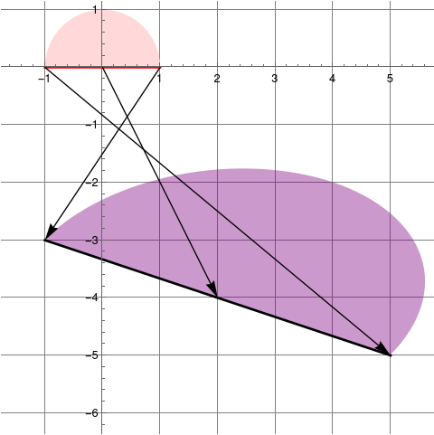
Now we plot the region after given affine transformation
We improve this plot by adding arrows to show how points are transformed.
This confirms that ratio of areas remain the same upon affine transformations.
■
End of Example 5
Affine Space (do you mean a fine space?)
Affine spaces provide a better framework for dealing with geometric object. In particular, it is possible to work with points, curves, surfaces, etc., in an intrinsic manner, that is, independently of any specific choice of a coordinate system. In affine spaces, points and their properties are frame invariant.
Recall that the Cartesian product of two sets A and B, denoted
A × B, is the set of all ordered pairs (𝑎, b), where 𝑎 is in A and b is in B. Since our main object of interest is ℝ, the set of real numbers, its direct product ℝ² = ℝ × ℝ inherits a linear structure (we know which number is larger than the other) from field ℝ. This space provides the main historical example of the Cartesian plane in analytic geometry.
The set of all such pairs (i.e., the Cartesian product ℝ × ℝ, denoted by ℝ²) is assigned to the set of all points in the plane as well as to the set of all free vectors. All these three sets (the set of points on the plane, the set of 2-tuples, and the set of free vectors in ℝ²) are in one-to-one and onto correspondence between each other. Therefore, they traditionally are denoted by ℝ², and content specifies which of these sets is in use.
One can similarly define the Cartesian product of n sets, also known as an n-fold Cartesian product, which can be represented by an n-dimensional array, where each element is an n-tuple.
In Euclidean space, points and vectors are usually identified with n-tuples.
In particular, a Euclidean plane contains points P(x, y) and vectors v(x, y) simultaneously because they both have the same coordinates.
In computer graphics, the main problem is to render or display a three-dimensional objects (or models) by projecting or mapping them into two-dimensional images.
Then the two-dimensional data must be converted into a form that the computer
can display (rasterization) and then be displayed. This requires a viewpoint or direction of projection and a viewing or projection plane. Fortunately, a monitor is just a two-dimensional array of finite number of pixels, short for picture elements.
The practical situation with rastering data in computer graphics shows that we
need to distinguish points from vectors. It is important because points and vectors have some mutually exclusive properties. A point has location but no extent while a vector in ℝ³ has both direction and magnitude (norm) but
its location is independent.
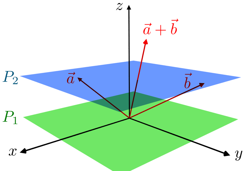
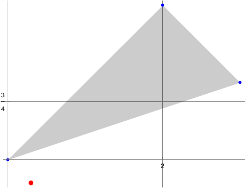
Example 6:
In order to visualize an affine plane, we
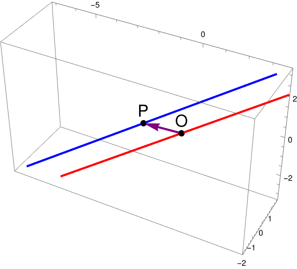
consider a 2D plane ℝ² inside ℝ³. In order to separate points from vectors, we choose two planes, one for points and another one for vectors, as in the picture below. We'll call the green one the vector space V ≌ ℝ² and the blue one as the point plane A. The plane V passes through the origin since it is a vector space, but the blue plane A does not. However, the inhabited set A looks almost exactly the same as V, having the exact same, flat geometry, and in fact A and V are simply translates of one another. This plane A is a classical example of an affine space. Later you will see
that any affine space is isomorphic to the affine space generated by V. You will learn in Part 3 that A is a coset of V.
Figure 3: Wrong model of affine plane from Wikipedia.
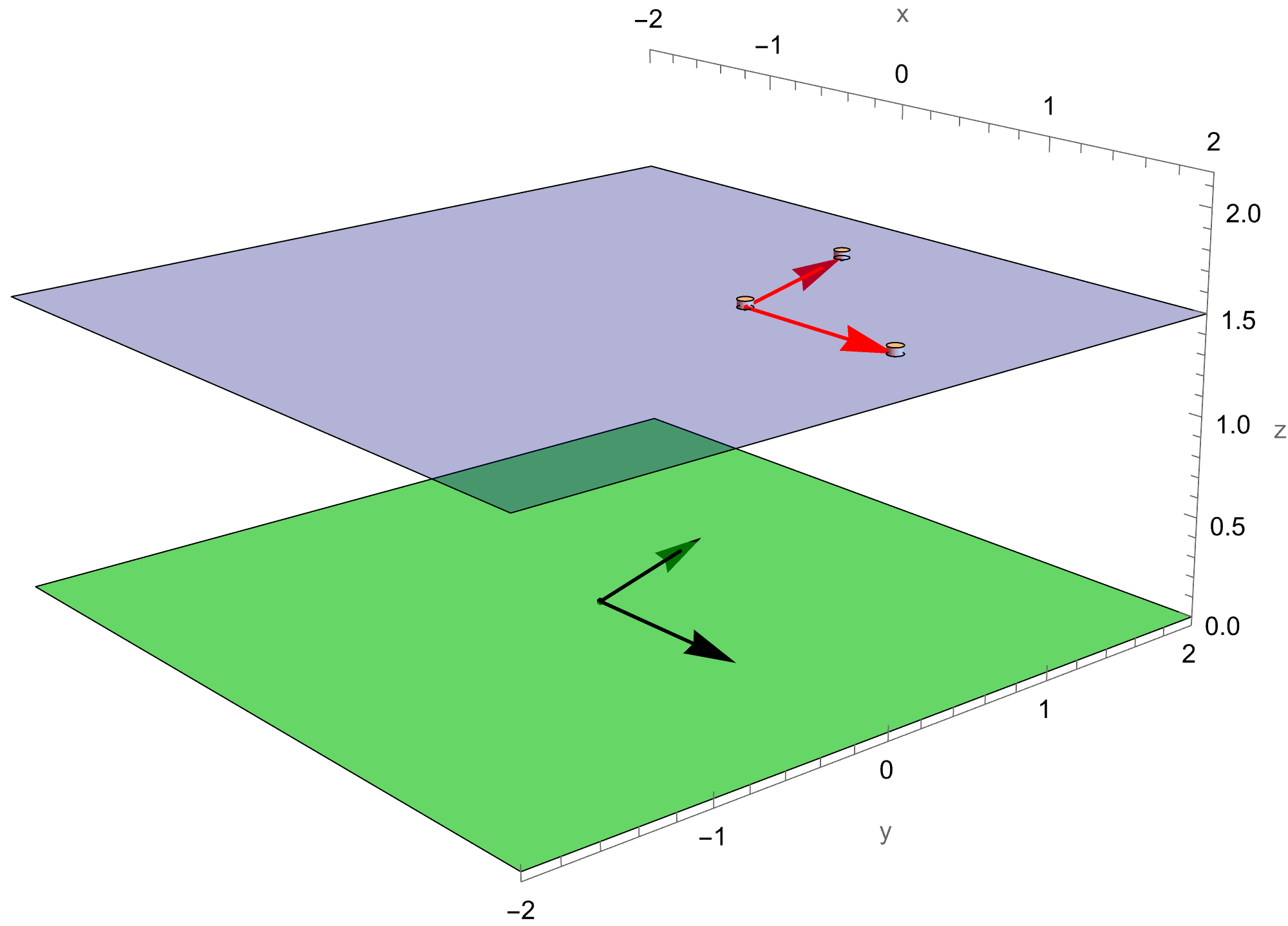
Figure 4: Affine plane.
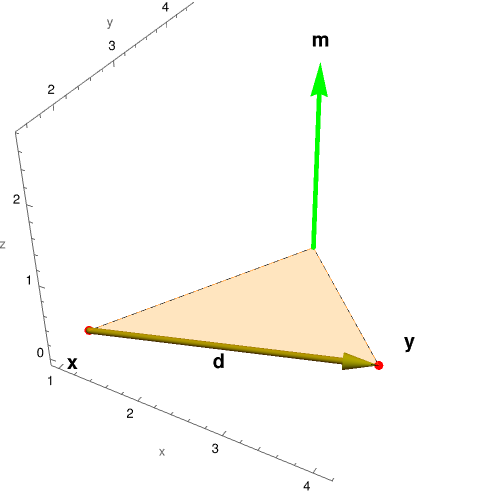
The Wolfram code below produces Figure 4 above.
Clear[x, y, p, a, b, c, plt1];
Define the vectors
x = {{0, 0, 0}, {1, 0, 0}};
y = {{0, 0, 0}, {0, 1, 0}};
Define the starting point for the red arrows on the green plane
p = {0.0, 0.0, 0.0};
Define two vectors a and b on the blue plane, not parallel to the\ x, y, or z, and making 110 degrees with each other.
a = p + {Cos[0], Sin[0], 0};
b = p + {Cos[110 Degree], Sin[110 Degree], 0};
Calculate the sum of the two vectors
c = p + (a - p) + (b - p);
Define the transformation : a translation moving the vectors to the blue plane in the z - direction
transformZ = TranslationTransform[{0, 0, 1.5}];
Define the lateral displacement : a translation moving the\ vectors in the x - y plane.
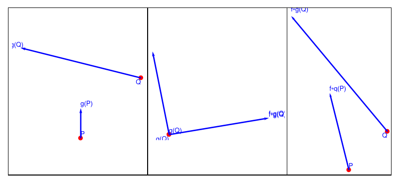
The left picture shows an attempt to introduce vector structure in the inhabited set A. Let T : A ↦ V be a translation of the point set to the vector space. You may try to define addition of two points as
However, the resulting vector (P(+)Q) does not belong to the inhabited set A. It is impossible to introduce a vector structure into an inhabited set of points---it is not a vector space because it has no algebraic structure. The basic idea of affine space is inherited from physics where forces (vectors) are acting on point objects to move them into another position (point again).
■
End of Example 6
Now we are ready to make a general definition of an affine space. We start with a succinct version
according to Wikipedia for pure mathematicians.
Practitioners prefer to use a more elaborate definition. There are two versions of this definition using the action of vectors on points due to either "addition" of points and vectors or "subtraction" of points.
We present both versions to please everyone.
In context of linear algebra, an affine space is a set of points A equipped with a set of transformations (that is bijective mappings); the translations, which form a vector space (over a given field, commonly the set of real numbers), such that for any given ordered pair of points there is a unique translation sending the first point to the second one; such translation is also called the action of a vector on a point. The composition of two translations is their sum in the vector space of the translations.
An affine space over a field 𝔽 is a triple (A, V, +), consisting of a vector space V over a field 𝔽, a set A whose elements are called points, and an external binary operation A × V ↣ A : (𝑎, v) ↦ 𝑎 + v, satisfying the following axioms:
(𝑎 + v) + u = 𝑎 + (v + u) for all 𝑎 ∈ A and ∀ v, u ∈ V;
𝑎 + 0 = 𝑎 for all 𝑎 ∈ A;
for any two points 𝑎, b ∈ A, there exists a unique vector x ∈ V, so that b = 𝑎 + x.
It is customary to denote points as n-tuples and vectors as column or row vectors. Then action of vector x on point 𝑎 can be written as
Every finite dimensional linear space V has an affine structure (V, V, +) inherited by vector addition from V, see Example 8 for details. We will refer
to the affine structure (V, V, +) on a vector space V as the canonical (or natural) affine structure on V. In particular, the vector space ℝn can
be viewed as the affine space (ℝn, ℝn, +). We often call the triple (A, V, +) or pair (A, V) an affine
space, omitting other terms and denote it as 𝔸. The mapping A ↣ A : P ↦ P + x is called a translation by
vector x or action of vector x on point P.
Any vector space V has an affine space structure specified by choosing the inhabited set to be V and letting "+" be addition in the vector space V.
Example 7:
Any finite dimensional vector space V has an affine space structure specified by choosing the inhabited set A = V and letting d be subtraction in the vector space V. We will refer
to the affine structure (V, V, d) on a vector space V as the canonical affine structure on V. In particular, the vector space ℝn can be viewed as the affine space (ℝn, ℝn, d), denoted by 𝔸n. The affine space 𝔸n is called the real affine space of dimension n.
Recall that a frame in ℝ³ (we restrict ourselves with n = 3 for simplicity) is a pair consisting of the point O (called the origin) and an ordered basis ε = [e₁, e₂, e₃]. For example, the standard frame in ℝ³ has origin O = (0, 0, 0) and the basis of three vectors e₁ = (1, 0, 0) = i,
e₂ = (0, 1, 0) = j, and e₃ = (0, 0, 1) = k. The position of a point P is then defined
by the “unique vector” from O to P. This approach identifies point P(p₁, p₂, p₃) with corresponding vector
\( \displaystyle \quad {\bf x} = \overline{OP} = \left( p_1 , p_2 , p_3 \right) . \)
Hence, in a standard frame of ℝ³, points and vectors are identically represented by triples of real numbers. However, if we choose another frame with different origin Ω = (ω₁, ω₂, ω₃), but with the same basis vectors ε, points and position vectors are no longer identified. This time, the point P = (p₁, p₂, p₃) is defined by by two position vectors:
\[
OP = \left( p_1 , p_2 , p_3 \right)
\]
in frame (O, ε) and
\[
\Omega P = \left( p_1 - \omega_1 , p_2 - \omega_2 , p_3 - \omega_3 \right)
\]
in frame (Ω, ε). This is because
\[
OP = O\Omega + \Omega P \qquad \mbox{and} \qquad O\Omega = \left( \omega_1 , \omega_2 , \omega_3 \right) .
\]
In the second frame (Ω, ε), points and position vectors are no longer identical.
■
End of Example 7
It is convenient to denote the vector v ∈ V for which Q = P + v by \( \displaystyle \quad \overline{PQ} \quad \mbox{or} \quad \vec{PQ} . \quad \mbox{or} \quad Q - P , \quad\) or just PQ. So the difference of two points is just an abbreviation of vector v such that Q = P + v. Based on this difference operation, we give an equivalent definition of affine space.
An affine space with vector space V is a nonempty set A of
points and a vector valued map d : A × A ↦ V called a difference function, such
that for all P, Q, R ∈ A
d(P, Q) + d(Q, R) = d(P, R), Chasles's identity;
the restricted map d₁ = d{P}×A : {P} × A ↦ V defined as mapping (P, Q) ↦ d(P, Q) is a bijection. d(P, Q) is referred to as a translation vector.
The first condition (i) is just the usual “parallelogram property” of the addition of vectors. From the second condition, it follows that for every pair of points P and Q from A, there exits a unique vector v ∈ V such that P + v = Q.
Lemma 1:
In an affine space (A, V, d) with difference function d we have
d(P, P) = 0 for all points P ∈ A,
d(P, Q) = −d(Q, P) for all points P, Q ∈ A.
d(P, P) = 0 for all points P ∈ A,
The difference function d maps two points P and Q in the affine space to a vector in the vector space V. By definition, the vector d(P, P) represents the difference between the point P and itself. In any affine space, the difference between a point and itself is the zero vector 0. Hence, d(P, P) = 0.
d(P, Q) = −d(Q, P) for all points P, Q ∈ A.
In three dimensional space, the vector d(P, Q) represents the direction and distance from point P to point Q. Similarly, d(Q, P) represents the direction and distance from point Q to point P. By the properties of vector spaces, reversing the direction results in the negative of the original vector. Thus, d(P, Q) = −d(Q, P). This property is extended for arbitrary vector space.
Example 8:
Let us consider the subset A of 𝔸³ consisting of all
points (x, y, z) satisfying the equation
\[
x^2 + y^2 - z = 0 .
\]
The set of points A is a paraboloid of revolution, with axis Oz. The surface A can be made into an official affine space by defining the action of addition of points and vectors (which is equivalent to the difference operation d) s : A × ℝ² → A
of ℝ² on A defined such that for every point (x, y, x² + y²) on A and any vector v = (v, u) ∈ ℝ²,
\[
\left( x, y , x^2 + y^2 \right) + \begin{bmatrix} v \\ u \end{bmatrix} = \left( x + v , y + u , (x+v)^2 + (y+u)^2 \right) .
\]
■
End of Example 8
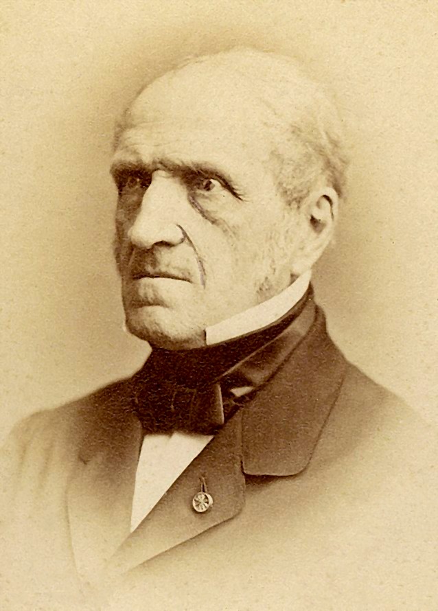
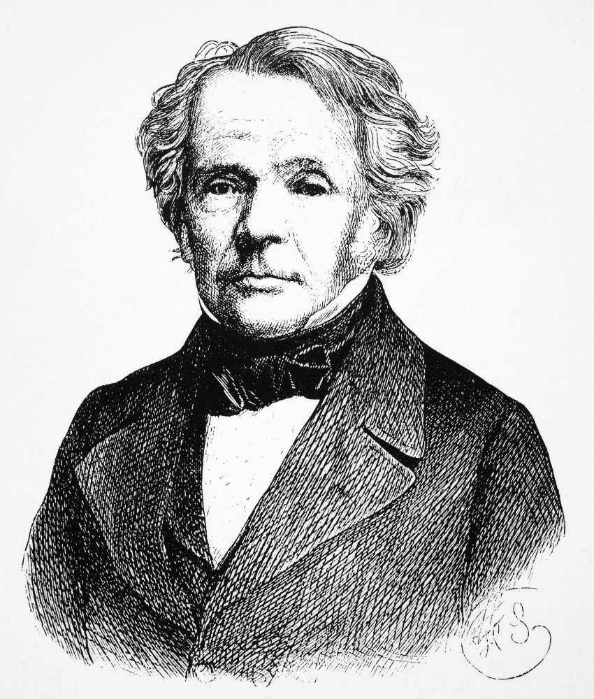
Michel ChaslesMichel Floréal Chasles (1793--1880) was a French geometer who published in 1837 the book Aperçu historique sur l'origine et le développement des méthodes en géométrie ("Historical view of the origin and development of methods in geometry"), a study of the method of reciprocal polars in projective geometry. Chasles was elected a Foreign Honorary Member of the American Academy of Arts and Sciences in 1864. In 1865 he was awarded the Copley medal.
for any three points 𝑎, b, c in the inhabited set A of an affine space (A, V, +).
In an affine space (A, V, d), for any three points P, Q, R ∈ A, and any real number λ addition of points and scalar multiplication is defined via
\[
\begin{split}
\left( P, Q \right) + \left( P, R \right) &= d^{-1} \left( d\left( P, Q \right) + d\left( P, R \right) \right) ,
\\
\lambda \left( P, Q \right) &= d^{-1} \left( \lambda\, d \left( \left( P, Q \right)\right) \right) .
\end{split}
\]
This vector space is the
tangent space to A at point P, denoted TP(A). For v ∈ TP(A) ≌ V, we denote P + d−1(v) as P + v.
Example 9:
Let P₀ = (x₀, y₀, z₀) be a point on a surface S ⊂ ℝ³, and let C be any curve passing through P₀ and lying entirely in S. If the tangent
lines to all such curves C at P₀ lie in the same plane, then this plane is called the tangent plane
to S at P₀.
For a tangent plane
to a surface S
to exist at a point on that surface, it is sufficient for the function
that defines the surface
to be continuously differentiable
at that point. If a surface is defined by a differentiable function z = f(x, y), and P₀ = (x₀, y₀, z₀) is a point on S, then the equation of the tangent plane at P₀ is given by
\[
z = f(x_0 , y_0 ) + f_x (x_0 , y_0 ) \left( x- x_0 \right) + f_y (x_0 , y_0 ) \left( y- y_0 \right) .
\tag{9.1}
\]
To see why this formula is correct, let’s first find two
lines tangent to the surface S. The equation of the tangent
line to the curve that is represented by the intersection of S with the vertical trace
given by x = x₀ is z = f(x₀, y₀) + fy(x₀, y₀)(y − y₀). Similarly, the equation of the tangent
line to the curve that is represented by the intersection of S with the vertical trace
given by y = y₀ is z = f(x₀, y₀) + fx(x₀, y₀)(x − x₀). A parallel vector to the first tangent line is
a = j + fy(x₀, y₀)k, a parallel vector to the second tangent line is b = i +
fx(x₀, y₀)k. We can take the cross product of these two vectors
\begin{align*}
{\bf a} \times {\bf b} &= \left( {\bf j} + f_y (x_0 , y_0 )\,{\bf k} \right) \times \left( {\bf i} + f_x (x_0 , y_0 )\,{\bf k} \right)
\\
&= \begin{vmatrix} {\bf i} & {\bf j} & {\bf k} \\ 0&1& f_y (x_0 , y_0 ) \\ 1&0& f_x (x_0 , y_0 ) \end{vmatrix}
\\
&= f_x (x_0 , y_0 )\,{\bf i} + f_y (x_0 , y_0 )\,{\bf j} - {\bf k} .
\end{align*}
This vector is perpendicular to both lines and is therefore perpendicular to the tangent plane. We can use this vector
as a normal vector to the tangent plane, which we denote as n = a × b/(∥a × b∥) (of unit length), along with the point P₀ = (x₀, y₀, z₀) in the equation for a plane:
\begin{align*}
{\bf n} \bullet \left( (x- x_0 )\,{\bf i} + (y - y_0 )\,{\bf j} + (z - f(x_0 , y_0 ))\,{\bf k} \right) &= 0 ,
\\
\left( f_x (x_0 , y_0 )\, {\bf i} + f_y (x_0 , y_0 )\,{\bf j} - {\bf k} \right) \bullet \left( (x- x_0 )\,{\bf i} + (y - y_0 )\,{\bf j} + (z - f(x_0 , y_0 ))\,{\bf k} \right) &= 0 ,
\\
f_x (x_0 , y_0 )\left( x - x_0 \right) + f_y (x_0 , y_0 ) \left( y - y_0 \right) - \left( z - f(x_0 , y_0 ) \right) &= 0.
\end{align*}
Solving this equation for z gives Equation (9.1).
As an example, let us choose a quadratic function f(x, y) = 3 x² − 5 xy − 7 y² + 4 x − 5 y + 1 at point (−2, 1). First, we calculate derivatives
\begin{align*}
f_x (x,y) &=6\,x - 5\,y + 4,
\\
f_x (-2,1) &= -13 ,
\\
f_y (x,y) &= -5 - 5 x - 14 y ,
\\
f_y (-2,1) &= -9 .
\end{align*}
Mathematica confirms calculations above.
Then Eq.(9.1) becomes
\[
z = 3 -13 \left( x+2 \right) -9 \left( y -1 \right) .
\]
Here is how Mathematica sees this. First, we define S, the surface function
Clear[f, x, y, z, fx, fy, P0, fx0, fy0];
f[x_, y_] := 3 x^2 - 5 x y - 7 y^2 + 4 x - 5 y + 1;
Then we compute partial derivatives
fx = Derivative[1, 0][f];
fy = Derivative[0, 1][f];
Defining Subscript[P, 0] requires our x and y values and the value of the function at those values (z)
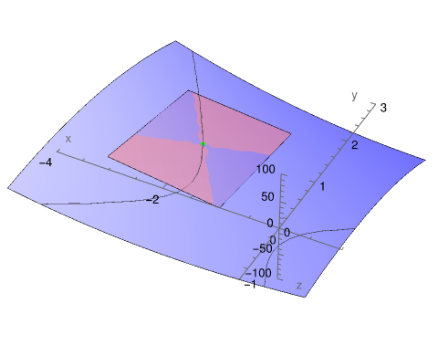
We are now in a position to plot. Note that, while the tangent plane is indeed tangent to the surface at P₀, it intercepts the surface in other places. So, we plot the surface and tangent plane using a smaller range for the tangent plane.
The two parabolas you see in the plot are the vertical traces of the surface, which are obtained by intersecting the surface z = f(x,y) with the planes x = x₀ and y = y₀. The equations for these parabolas can be derived by substituting these values into the surface equation.
Given the surface equation:
z==f(x,y)==3x^2-5xy-7y^2+4x-5y+1
The two parabolas are:
1. Vertical trace at x = x₀ ==-2: z = f(-2,y) == 3(-2)^2-5(-2)y-7y^2+4(-2)-5y+1
Simplifying the expression:
z==12+10y-7y^2-8-5y+1
z==-7 y^2+5y+5
So, the equation for the first parabola is:
z==-7 y^2+5y+5
2. Vertical trace at y = y₀ ==1:
z==f(x,1)==3x^2-5x(1)-7(1)^2+4x-5(1)+1
Simplifying the expression:
z==3x^2-5x-7+4x-5+1
z==3x^2-x-11
So, the equation for the second parabola is:
z==3x^2-x-11
Thus, the equations for the two parabolas are:
1. z==-7 y^2+5y+5
2. z==3x^2-x-11
These are the vertical traces of the surface at x==-2 and y==1, respectively.
■
End of Example 9
As the notion of parallel lines is one of the main properties that is independent of any metric, affine geometry is often considered as the study of parallel lines.
Affine Sets and Combinations
In this subsection, we consider only field ℝ of real numbers and
finite dimensional vector spaces over ℝ.
To motivate understanding of affine combinations, we recall the vector equations of lines and planes in ℝ³ that do not necessarily pass through the origin (see section in this chapter). You can skip the following example if you know this material.
Example 10:
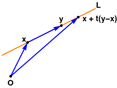
Let us consider the line L in ℝ³
through the distinct points x, y ∈ ℝ³. Geometrically, we can reach each point on this line
by starting at the origin, traveling to the tip of the vector x (viewed as an arrow starting
at 0), then following some scalar multiple t(y − x) of the direction vector y − x for the line
(where t ∈ ℝ). Algebraically, the line consists of all vectors x + t(y − x) as
t ranges over ℝ. Restating this,
\[
L = \left\{ t\,{\bf y} + \left( 1- t \right) {\bf x} \ : \ t \in \mathbb{R}\right\} .
\]
In other words, L consists of all affine combinations of x and y. Recall that a linear combination of two vectors includes all points
\( \displaystyle \quad t\,{\bf y} + s \,{\bf x} , \quad \) where t, s ∈ ℝ, without constraint s = 1 − t.
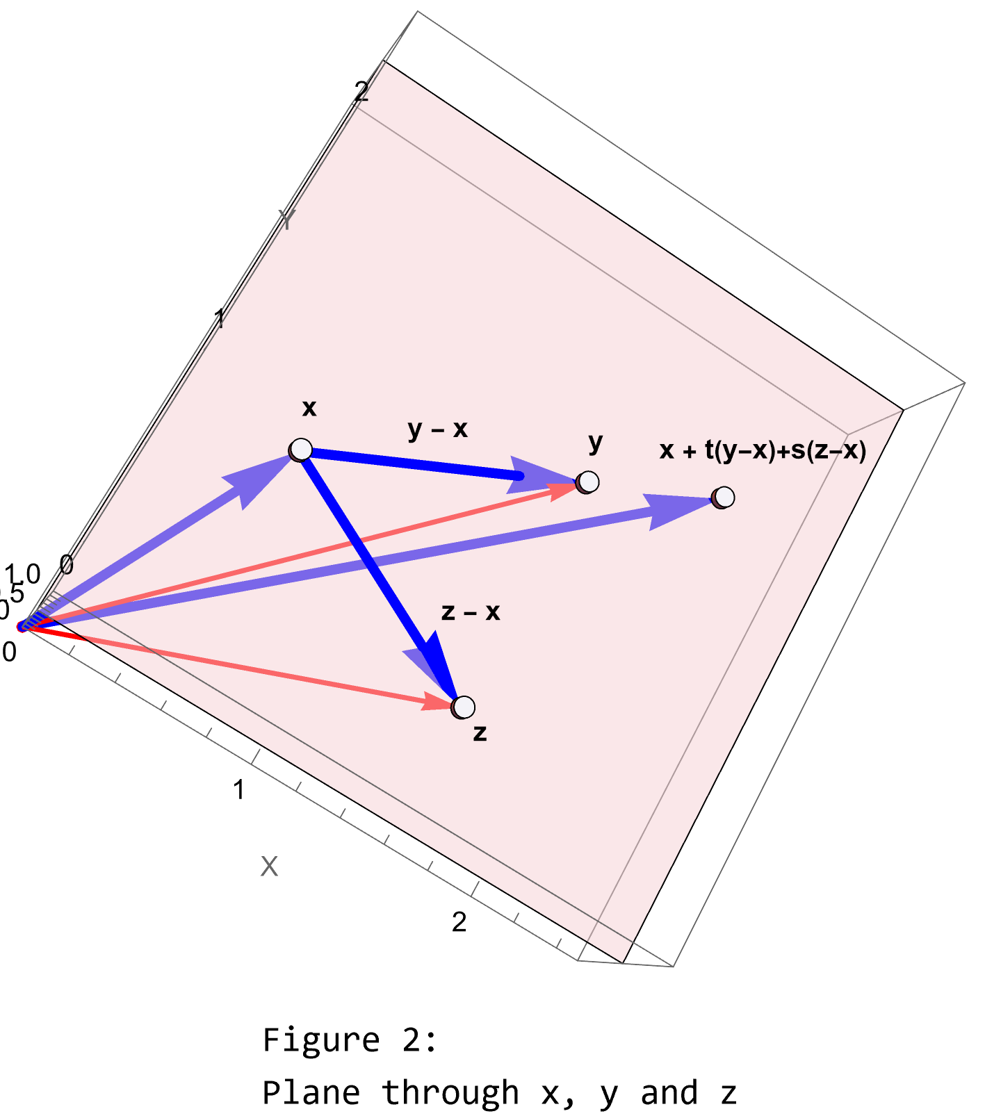
Similarly, consider the plane P in ℝ³ through three non-collinear points x, y, z ∈ ℝ³.
As in the case of the line, we reach arbitrary points in P from the origin by going to the tip
of x, then traveling within the plane some amount in the direction y − x and some other
amount in the direction z − x. Algebraically, we have
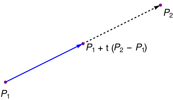
As a further example, we consider two points P₁ and P₂ in a two-dimensional affine space. The following expression
\[
P = P_1 + t \left( P_2 - P_1 \right)
\]
makes sense because the difference P₁ − P₂ is a vector, and thus so is t(P₁ − P₂). Therefore, P is the sum of a point and a vector which is again a point in the inhabited set. This point P lies on the line going through two other points P₁ and P₂. Note that if 0 ≤ t ≤ 1, then P is somewhere on the line segment joining P₁ and P₂.
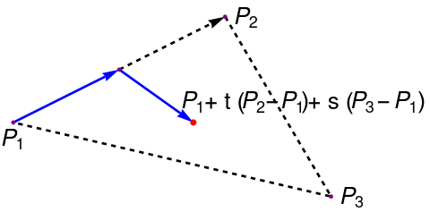
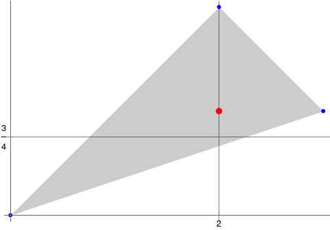
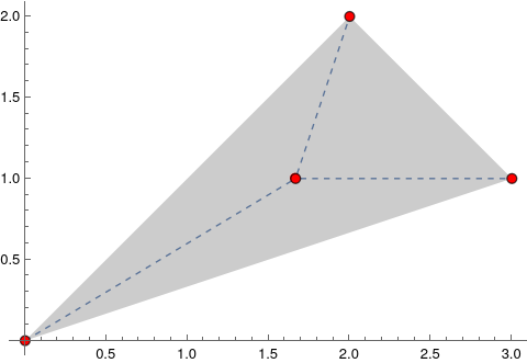
Now we consider three points; the following figure shows a combination of these points:
\[
P = \alpha_1 P_1 + \alpha_2 P_2 + \alpha_3 P_3 , \qquad \alpha_1 + \alpha_2 + \alpha_3 = 1.
\]
In order to understand a fundamental concept of linear combination in affine geometry, we recommend to open the following example.
Example 11:
Let us consider the affine transformation applied to column vectors:
\[
\mathbb{F}^{n\times 1} \ni \mathbf{x} \longrightarrow f({\bf x}) = {\bf A}\,{\bf x} + \mathbf{b} ,
\tag{11.1}
\]
where A is an m-by-n real matrix and b is a given m-column vector. We check whether this (arbitrary) affine transformation transfers affine combinations into another affine combination.
For arbitrary two real scalars α, β ∈ ℝ, we have
\[
f \left( \alpha {\bf x} + \beta {\bf y} \right) = \alpha\,{\bf A}\,{\bf x} + \beta \,{\bf A}\,{\bf y} + \mathbf{b} ,
\]
for arbitrary column vectors x and y. If we want this affine transformation to preserve linear combination, we need to satisfy the identity
\[
f \left( \alpha {\bf x} + \beta {\bf y} \right) = \alpha\,f \left( {\bf x} \right) + \beta\,f \left( {\bf y} \right)
\]
or
\[
\alpha\,{\bf A}\,{\bf x} + \beta \,{\bf A}\,{\bf y} + \mathbf{b} = \alpha \left( {\bf A}\,{\bf x} \right) + \beta \left( {\bf A}\,{\bf y} \right) + \left( \alpha + \beta\right) \mathbf{b} .
\]
The latter identity is true only when
\[
\alpha + \beta = 1.
\tag{11.2}
\]
Therefore, we conclude that the affine transformation (11.1) preserves linear combination of two points only when weights α and β satisfy the condition (11.2).
It is straight forward to verify that a linear combination of n column vectors x₁, x₂, … , xn with weights c₁, c₂, … , cn is preserved by affine transformation (11.1) only when these weights satisfy the condition
\[
\sum_{i=0}^n c_i = 1 .
\]
■
End of Example 11
Consider a system of n+1 particles, located at x₀, x₁, … , xn and with masses w₀, w₁, … , wn.
It is then well-known from physics that the center of mass or barycentre of this
particle system is the unique point x which satisfies
\[
x = \frac{\sum_{i=0}^n w_i x_i}{\sum_{i=0}^n w_i} .
\]
Clear[x, n, w, i]; \( \displaystyle \quad \mbox{Solve}\left[ \sum_{i=0}^n w_i * \left( x - x_i \right) == 0, \ x \right] \)
Sum[w[i]*x[i], {i, 0, n}]/Sum[w[i], {i, 0, n}]
This physical situation can be reformulated mathematically as follows. For a given fixed set of distinct locations or nodesx₀, x₁, … , xn and an arbitrary point x,
does there exist some masses or weights w₀, w₁, … , wn, such that x is the barycentre \( \displaystyle \quad x = \sum_j w_j x_j , \qquad \sum_j w_j = 1 , \quad \) of
the corresponding particle system?
Here is Wolfram code which answers that question and animates two bodies with the same masses.
First we define the initial positions of the two bodies
x0 = {0, 0};
x1 = {2, 0};
Since the masses are equal we can just make them 1
w0 = 1;
w1 = 1;
Calculate the barycenter
barycenter = (w0*x0 + w1*x1)/(w0 + w1);
Define the time-dependent positions of the two bodies and animate
Similar code can produce behavior for two bodies with unequal masses
Two bodies with similar masses.
Two bodies with distinct masses
Two bodies with the same masses.
A. Möbius was probably the first to answer this question in full generality. He
showed that for particle systems in ℝm such weights always exist for any x ∈ ℝm,
as long as the number of particles is greater than the dimension, that is, for n ≥ m.
Möbius called the weights w₀(x), w₁(x), … , wn(x) the barycentric coordinates of x with
respect to nodes x₀, x₁, … , xn.
It is clear that barycentric coordinates are homogeneous in the sense that they
can be multiplied with a common non-zero scalar and still satisfy
We can generalize this to define an affine combination of an arbitrary number of points. If P₁, P₂, … ,Pn
are points and w₁, w₂, … ,wn are scalars such that w₁ + w₂+ ⋯ + wn = 1, then
\[
w_1 P_1 + w_2 P_2 + \cdots + w_n P_n
\]
is defined to be the point in the inhabited set because
This equation is meaningful, as P₂ − P₁ is a vector, and thus so is its multiple w₂(P₂ − P₁).
Lemma 2:
Given an affine space A, let {𝑎i}i∈I be a family of points in A, and let {λi}i∈I be a family of scalars. For any two points 𝑎, b ∈ A, the
following properties hold:
If \( \displaystyle \quad \sum_{i\in I} \lambda_i = 1 , \quad \) then
\[
a + \sum_{i\in I} \lambda_i \,\vec{a\,a_i} = b + \sum_{i\in I} \lambda_i \,\vec{b\,a_i} .
\]
Example 12:
Let us consider three points in two-dimensional space ℝ² with respect to some frame:
\[
a (0, 0), \qquad b(2, 2), \qquad c (3, 1) .
\]
Of course, the expressions for points are not written accurately (from mathematician prospective), but lazy people like me use this informal notation. These points should be written as
\[
P_1 = O + a , \qquad P_2 = O + b , \qquad P_3 = O + c .
\]
Using these three points, we determine three other points
\[
p_1 = \frac{1}{4}\, a + \frac{1}{4}\, b + \frac{1}{2}\, c , \quad
p_2 = \frac{1}{3}\, a + \frac{1}{3}\, b + \frac{1}{3}\, c , \quad
p_3 = a - b + c .
\]
Now we explore Mathematica. First, we define points.
Clear[a, b, c, p1, p2, p3];
a = {0, 0};
b = {2, 2};
c = {3, 1};
Create triangle from these points that are marked now blue,
Note that for p1 we divide b by 4, so we have b/4. Now we modify this point p1 by introducing a coefficient (0,1) multiplier, .5 − t. Then upon changing t, we obtain new barycenters depending on the value of t. Because variable names are re-used below the following animation later in the notebook, the animation will change upon evaluation of later cells.
Generally speaking, a sum P + Q of two points in the inhabited set A is meaningless (except when A = V is a vector space itself).
By Lemma 2, for any family of points
(𝑎i)i∈I in the inhabited set A, for any
family (λi)i∈I of scalars such that
\( \displaystyle \quad \sum_{i \in I} \lambda_i = 1 , \quad \) the point
\[
x = a + \sum_{i\in I} \lambda_i \,\vec{a\, a_i}
\]
is independent of the choice of the origin 𝑎 ∈ A.
In this form, the values (λ₀, λ₁, …., λn) are called the barycentric coordinates of x relative to the
points 𝑎₀, 𝑎₁, … , 𝑎n.
The restriction on weight coefficients to be \( \quad \sum_{i \in I} \lambda_i = 1 \quad \) makes definition of affine combination frame free. Note that
the notion of linear combination of vectors in a vector space is basis independent.
This property motivates the following definition.
For any family of points (𝑎i)i∈I in the inhabited set A, for any family
(λi)i∈I of scalars such that \( \displaystyle \quad \sum_{i \in I} \lambda_i = 1 , \quad \) and for any point
𝑎 ∈ A
\[
a + \sum_{i\in I} \lambda_i \,\vec{a\, a_i}
\]
(which is independent of 𝑎 ∈ A, by Lemma 2) is called the barycenter (or barycentric combination, or affine combination) of the points (𝑎i)i∈I assigned
the weights λi, and it is denoted by
\[
\sum_{i\in I} \lambda_i \, a_i \qquad \left( \sum_{i \in I} \lambda_i = 1 \right) .
\]
This allows us to make the following observation.
A sequence 𝑎₀, 𝑎₁, … , 𝑎n of n+1 points in n dimensional space is affinely independent if and only if each point x ∈ A (= ℝn) can be written uniquely as an affine combination of them, i.e.,
\[
x = \sum_j \lambda_j (x)\, a_j , \qquad \sum_{0 \le j \le n} \lambda_j (x) = 1 .
\]
The functions λj, so defined, are called barycentric coordinates of point x.
We can use linear subspaces of V to build more examples of affine sets in V. Let W be a fixed
linear subspace of V. Since W is closed under all linear combinations of its elements, which
include affine combinations as a special case, W is an affine subset of V. For any vector u ∈ V, its translation u + W = { u + w : w ∈ W } by subspace W is an affine set.
Theorem 3:
For every nonempty affine set X in a finite dimensional vector space
V, there exists a unique linear subspace W in V, known as the direction subspace, such that X = u + W = { u + w : w ∈ W} for some (possibly not unique) u ∈ V.
You will learn in Part 3 (Quotient spaces) that the set u + W is called the coset
Fix a nonempty affine set X in V, and fix u ∈ X. Define W = −u + X. On one
hand, W is an affine set, being a translate of the affine set X. On the other hand, u ∈ X
implies 0 = −u + u ∈ W. By the result preceding the theorem, W is a linear subspace, and
evidently u + W = u + (−u + X) = X. We now prove uniqueness of the linear subspace W. Say X = u + W = v + W₁ for some u, v ∈ V and linear subspaces W and W₁. Since
0 ∈ W and 0 ∈ W₁, u and v belong to X. Then v = u + w for some w ∈ W, hence W₁ = −v + X = (−v + u) + W = −w + W = W. (The last step uses the fact that
x + W = W for all x in a subspace W.)
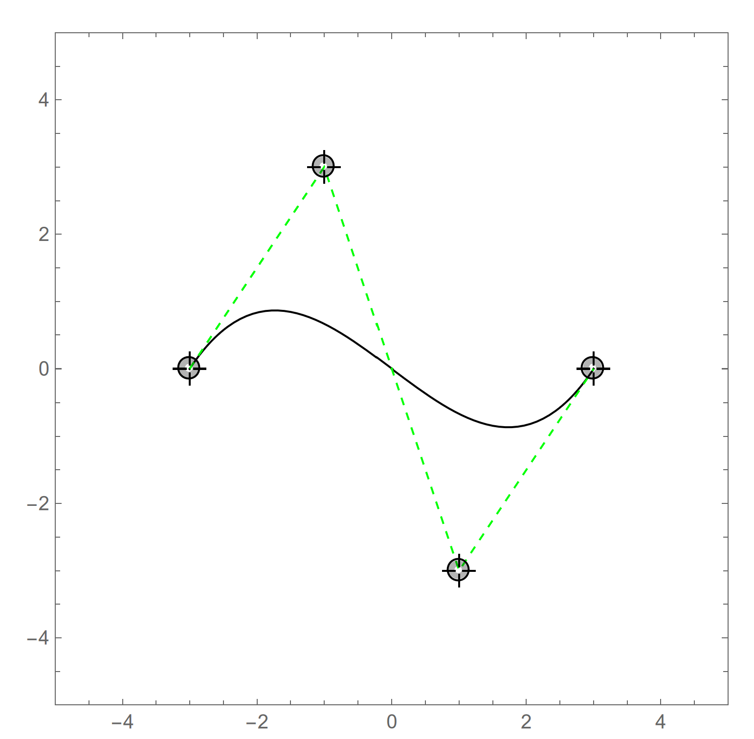
Example 13:
This example demonstrates that an arbitrary polynomial curve can be defined as a set of barycenters of a fixed number of points. For example, let (𝑎, b, c, d) be a
sequence of points in 𝔸². Observe that
\[
\left( 1- t \right)^3 + 3t \left( 1 - t \right)^2 + 3t^2 \left( 1 - t \right) + t^3 = 1
\]
because the sum on the left-hand side is obtained by expanding
\[
\left( 1 + (1-t) \right)^3 = \sum_{i=0}^3 \binom{3}{i} t^i \left( 1 - t \right)^{3-i} = 1
\]
using the binomial formula. Thus,
\[
\left( 1- t \right)^3 a + 3t \left( 1 - t \right)^2 b + 3t^2 \left( 1 - t \right) c + t^3 d
\]
is a well-defined affine combination. Then, we can define the curve F : 𝔸 → 𝔸² such that
\[
F(t) = \left( 1- t \right)^3 a + 3t \left( 1 - t \right)^2 b + 3t^2 \left( 1 - t \right) c + t^3 d
\]
Such a curve is called a cubic Bézier curve, and (𝑎, b, c, d) are called its control
points.
The mathematical basis for Bézier curves—the Bernstein polynomials—was established in 1912, but the polynomials were not applied to graphics until some 50 years later when mathematician Paul de Casteljau (1930--2022) in 1959 developed de Casteljau's algorithm, a numerically stable method for evaluating the curves, and became the first to apply them to computer-aided design at French automaker Citroën.
Note that the curve passes through 𝑎 and d, but generally not through b and c. For example, a Bézier curve can be used to specify the velocity over time of an object such as a cursor moving from A to B, rather than simply moving at a fixed number of pixels per step.
The Bézier curve can be constructed using
the de Casteljau algorithm. Although the algorithm is slower for most architectures when compared with the direct approach, it is more numerically stable.
Wolfram implemented de Casteljau's algorithm in a special build-in command: BezierCurve. Here is an illustration from the Mathematica Documentation. Use your cursor to drag the points about to see how it operates.
Since the direction subspace of an affine set X is uniquely determined by X, we can define the affine dimension of X (written dim(X)) to be the vector-space dimension of its direction subspace. For instance, points, affine lines, affine planes, and affine hyperplanes
have respective affine dimensions 0, 1, 2, and n − 1. The affine dimension of ∅ is undefined.
Theorem 4:
A subset of 𝔽n is an affine set if and only if it is the solution set to
a system of linear equations over 𝔽.
If S ⊆ 𝔽n is an affine set, it has the form S = b + W, where W is a subspace of 𝔽n and b is a vector in 𝔽n. Given such a set, let W₁ be a direct complement to W in 𝔽n. Note that we can assume b is in W₁.
Let A be the standard matrix representation of the projection onto W₁ along W. For w₁ in W₁ and w in W, we have
\[
{\bf A} \left( {\bf w}_1 + {\bf w} \right) = {\bf w}_1 .
\]
In particular, NullSpace(A) = W and A x = b. Lemma 2 (the general solution of A x = b is the sum of a particular solution and the general solution of the homogeneous equation) in section thus ensures that S is the
solution set to A x = b. This completes the proof in one direction.
The same Lemma 2 gives us the proof in the other direction.
Example 14:
Let us now consider data f₀, f₁, … , fn corresponding to the nodes x₀, x₁, … , xn and
possibly sampled from some function f : ℝm → ℝ, that is, fi = f(xi) for i = 0, 1 … , n.
The barycentric interpolant of this data is then given by
\[
F(x) = \sum_{0 \le i \le n} b_i (x)\, f_i .
\tag{14.1}
\]
The function F : ℝm → ℝ interpolates the data fi at xi for i = 0, 1 , … , n, and we require that this interpolation should be exact for linear functions:
\[
\sum_{0 \le i \le n} b_i (x) = 1 \qquad\mbox{and} \qquad \sum_{0 \le i \le n} b_i (x)\, x_i = x .
\]
This means that when data fi at xi
are sampled from a linear polynomial f, the interpolation (14.1) is exact: F(xi) = f(xi) for i = 0, 1 , … , n.
In particular, if we have two nodes
x₀, x₁, the two
functions b₀, b₁ : ℝ → ℝ are
\[
b_0 (x) = \frac{x_1 - x}{x_1 - x_0} , \qquad b_1 (x) = \frac{x - x_0}{x_1 - x_0}
\]
These functions form a barycentric basis with respect to x₀ and x₁ that lead to approximation
\[
F_1 (x) = \frac{x_1 - x}{x_1 - x_0} \, f\left( x_0 \right) + \frac{x - x_0}{x_1 - x_0} \, f \left( x_1 \right) .
\tag{14.2}
\]
In general, we have
\[
F_n (x) = \frac{\sum_{i=0}^n \frac{(-1)^i}{x - x_i} \, f\left( x_i \right)}{\sum_{i=0}^n \frac{(-1)^i}{x - x_i}} .
\tag{14.3}
\]
As a numerical example, we consider the sine function f(x) = sin(x) and two points x₀ = π/6 and x₁ = 3π/4. The corresponding two points barycentric interpolation reads as
\[
F_1 (x) = \frac{3\pi /4 -x}{7\pi /12} \, \frac{1}{2} + \frac{x - \pi /6}{7\pi /12} \, \frac{1}{\sqrt{2}} .
\]
Now we turn our attention to three point-interpolation. We again consider sine function and choose three points:
x₀ = π/6, x₁ = π/4, and x₂ = 3π/4. So we use formula (14.3) and ask Mathematica for help.
\[
F_2 (x) = \frac{\left( 9- 4\sqrt{2} \right) \pi^2 + 24 \left( -2 + \sqrt{2} \right) \pi x + 48 x^2}{10 \pi^2 -48 \pi x + 96 x^2} .
\]
For Mathematica, using the equations (14.3), we begin by defining the nodes.
Previously (see opening subsection of this web page) we defined affine transformation as \( \displaystyle \quad
\mathbb{F}^{n\times 1} \ni \mathbf{x} \longrightarrow f({\bf x}) = {\bf A}\,{\bf x} + \mathbf{b} \quad \)
for some column vector b ∈ 𝔽m×1
or \( \displaystyle \quad
\mathbb{F}^{1\times m} \ni \mathbf{v} \longrightarrow f({\bf v}) = {\bf v}\,{\bf A} + \mathbf{w} \quad \) for row vectors. Its generalization for arbitrary affine spaces is due to A. Grothendieck (1928--2014), who realized that an affine map should consist of two parts: one transformation for inhabited sets and another one for corresponding vector spaces.
Let 𝔸 = (A, V, +) and 𝔹 = (B, U, +) be two affine spaces over the same field 𝔽. The pair (f, Df), where f : A ↣ B and Df : V ⇾ U, satisfying the following conditions:
Df is a linear mapping from V into U;
for any two points P, Q from the inhabited set A,
\[
f(Q) - f(P) = D\,f(Q - P) \in U .
\]
is called an affine mapping of the first space into the second space.
Df or D(f) is the linear part of the affine mapping f. If affine transformation is given by \( \displaystyle \quad \mathbf{v} \longrightarrow f({\bf v}) = {\bf v}\,{\bf A} + \mathbf{w} ,\quad \) then Df is just matrix A. Since Q − P runs through all vectors in V when Q, P ∈ A, , the linear part Df is defined with respect to f uniquely. This makes it possible to denote affine mappings simply as f : 𝔸 ↣ 𝔹.
Formally, an affine map is a function (consisting of two parts) from one affine space to
another (which may be, and in fact usually is, the same space) that preserves affine combinations.
Example 15:
Any linear transformation T : V ⇾ U induces an affine mapping of the spaces (V, V, +) ↣ (U, U, +). For it, Df = f.
Transformation f : 𝔽n ↣ 𝔽n is an affine map for f(x) = A x + b because Df = A.
Any translation tx : A ↣ A, where tx(P) = P + x, is affine, and D(tx) = idV because
\[
t_{\bf x} (P) - t_{\bf x} (Q) = \left( P + {\bf x} \right) - \left( Q + {\bf x} \right) = P - Q .
\]
If f : 𝔸 ⇾ 𝔹 is an affine mapping and y ∈ U, then the mapping tx ∘ f : 𝔸 ⇾ 𝔹 is affine and D(tx ∘ f) = D(f). Indeed,
\begin{align*}
t_{\bf x} \circ f (P) - t_{\bf x} \circ f (Q) &= \left( t_{\bf x} (P) + {\bf x} \right) - \left( t_{\bf x} (Q) + {\bf x} \right)
\\
&= f(P) - f(Q) = Df(P-Q) .
\end{align*}
An affine function f : 𝔸 ↣ 𝔽 is defined as an affine mapping of 𝔸 into (𝔽, 𝔽, +). Thus, f assumes
values in 𝔽, while Df is a linear functional on V. Any constant function f is affine: Df = 0.
The identity mapping id : 𝔸 ↣ 𝔸 is an affine mapping. Indeed, P − Q = idV(P − Q). In particular, D(idA) = idV.
■
End of Example 15
It turns out that there is an alternative definition (which is of course equivalent to the previously used one) of affine mapping.
Given two affine spaces 𝔸 = (A, V, +) and 𝔹 = (B, U, +) under the same field of scalars. A function F : 𝔸 ↣ 𝔹 is an affine map if and only if for every family of points (𝑎i)i ∈ I and weights (λi)i ∈ I such that
∑i∈I λi = 1, we have
\[
F \left( \sum_{i\in I} \lambda_i a_i \right) = \sum_{i\in I} \lambda_i \, F \left( a_i \right) .
\]
In other words, F preserves barycenters.
Theorem 5:
Let f : 𝔸 ↣ 𝔹 be an affine map between two afine spaces 𝔸 = (A, V, +) and 𝔹 = (B, U, +) over the same field. Then there is a unique linear transformation Df : V ⇾ U such that
\[
f(a + {\bf x}) = f(a) + Df(\mathbf{x})
\]
for every 𝑎 ∈ A and every x ∈ V.
Let 𝑎 ∈ A be any point in the inhabited set. We claim that the map defined according t the identity
\[
Df(\mathbf{x}) = f(a)\,f(a + \mathbf{x}) \quad \iff \quad f(a + \mathbf{x}) = f(a) + Df(\mathbf{x})
\]
is a linear transformation Df : V ⇾ U
for every x ∈ V independently of point 𝑎 ∈ A.
Indeed, we can write
\[
a + \lambda \mathbf{x} = \lambda \left( a + \mathbf{x} \right) + \left( 1 - \lambda \right) a
\]
because 𝑎 + λx = 𝑎 + λ𝑎(𝑎 + x) + (1 − λ)𝑎𝑎, and also
\[
a + \mathbf{x} + \mathbf{y} = \left( a + \mathbf{x} \right) + \left( a + \mathbf{y} \right) - a
\]
Clear[f, a, v, \[Lambda]];
f[pt_] := pt + {1, 1} (* Example affine transformation *)
since 𝑎 + x + y = 𝑎 + 𝑎 (𝑎 + x) + 𝑎 (𝑎 + y) −𝑎𝑎. We also know that i>f preserves barycenters, so
\[
f\left( a + \lambda\mathbf{y} \right) = \lambda\, f(a + {\bf y}) + \left( 1 -\lambda \right) f(a) .
\]
Define the linear map Df:
Df[v_] := f[a+v] - f[a]
If we recall that \( \displaystyle \quad \sum_{i \in I} \lambda_i a_i \quad \) is the barycenter of a family points (𝑎i)i ∈ I and weights (λi)i ∈ I with \( \displaystyle \quad \sum_{i \in I} \lambda_i = 1 \quad \) iff
\[
b\,\mathbf{x} = \sum_j \lambda_j \,k{\bf a}_j \qquad \forall b \in V ,
\]
we get
\[
f(a)\,f(a+ \lambda{\bf v}) = \lambda\,f(a)\,f(a + {\bf v}) + \left( 1 - \lambda \right) f(a)\,f(a) = \lambda\, f(a)\,f(a+ \lambda{\bf v}) ,
\]
showing that
\[
Df(\lambda\mathbf{v}) = \lambda\,Df(\mathbf{v}) .
\]
We also have
\[
f(a+ \mathbf{u} + \mathbf{v}) = f(a+ \mathbf{u} ) + f(a+ \mathbf{v} ) -f(a) ,
\]
from which we get
\[
f(a)\,f(a + \mathbf{u} + \mathbf{v}) = f(a)\,f(a + \mathbf{u} ) + f(a)\,f(a + \mathbf{v} ) ,
\]
showing that
\[
Df(\mathbf{u} + \mathbf{v}) = Df(\mathbf{u}) + Df(\mathbf{v}) .
\]
Consequently, Df is a linear map.
For any other point b ∈ A, since
\[
b + \mathbf{v} = a + a{\bf b} + \mathbf{v} = a + a \left( a + \mathbf{v} \right) - aa + a{\bf b} .
\]
So b + u = (a + v) a + b, and since f _reserves barycenters, we get
\[
f(b + \mathbf{v}) = f(a + \mathbf{v}) - f(a) + f(b) ,
\]
which implies that
\begin{align*}
f(b)\,f(b+ {\bf v}) &= f(b)\,f(a + {\bf v}) - f(b)\, f(a) + f(b)\,f(b)
\\
&= f(a)\,f(b) + f(b)\, f(a + {\bf v})
\\
&= f(a)\,f(a+ {\bf v}) .
\end{align*}
Thus, f(b) f(b + v) = f(𝑎) f(𝑎 + v), which shows that the definition of Df does not depend on the choice of 𝑎 ∈ A.
The fact that Df is unique is
obvious: We must have Df(v) = f(𝑎) f(𝑎 + v).
Example 16:
Let us consider the affine transformation S : ℝ³ ↦ ℝ4 given by S(x) = A x + b, where
\[
\mathbf{A} = \begin{bmatrix} -2& 3& 5 \\ 3& 7& -1 \\ 5& 27& 7 \\ -9& 2&
16 \end{bmatrix}, \qquad {\bf b} = \begin{bmatrix} 3 \\ -6 \\ -12 \\ 15 \end{bmatrix} .
\]
First, we find solution A u = −b, so S(u) = 0, with the aid of Mathematica.
From solution given above, we can reconstruct the solution as a line given parametrically
\[
L = \left\{ \left( x, y, z \right) \ : \ x = -\frac{38}{23}\, t -\frac{39}{23} , \quad y = \frac{13}{23}\, t - \frac{3}{23} , \quad z = t , \quad \forall t \in \mathbb{R} \right\} .
\]
We can decompose L into a sum of two components: the first is the line L₀, which passes through origin; the second is a translation by a particular vector vp. To find the particular vector vp, notice that all we have to do is set t = 0 in the parametric definition of L given above, which yields
\( \displaystyle \quad {\bf v}_p = \left[ -\frac{39}{23} , \ -\frac{3}{23} , \ 0 \right] \quad \) Once we know vp, the line L₀ is simply the remaining portion of the solution
\[
L_0 = \left\{ \left( x, y, z \right) \ : \ x = -\frac{38}{23}\, t , \quad y = \frac{13}{23}\, t , \quad z = t , \quad \forall t \in \mathbb{R} \right\} .
\]
Clearly, L₀ is a line through the origin, and is thus a subspace of ℝ³. The line L can be realized as a translate of the line L₀ by the particular solution xp. Now let us plot these two lines along with the particular solution
xp.
The properties of affine transformations on points and vectors are summarized in the following theorem.
Theorem 6:
Let P and Q be points and u and v be vectors in an affine space 𝔸 = (A,V, d). Let F : 𝔸 ↣ 𝔹
be an affine transformation from 𝔸 to another affine space 𝔹 = (B, U, d). Then for any scalar α
DF(v) = DF(P − Q) = F(P) − F(Q) for v = P − Q,
F(P + αu) = F(P) + αDF(u) for any u ∈ V,
DF(u + v) = DF(u) + DF(v),
DF(αv) = αDF(v).
The first property is the definition of the linear part of an affine map.
The second property is a reformulation of Theorem 5.
Showing part (c) is straight forward if P and Q are points in 𝔸 such that u = P − Q and
v = Q − R and the head-to-tail axiom is applied several times.
\begin{align*}
F(\mathbf{u} - \mathbf{v}) &= F \left( (P - Q) + (Q - R) \right)
\\
&= F(P - R) = F(P) - F(R)
\\
&= F(P) - F(Q) + F(Q) - F(R)
\\
&= F(P - Q) + F(Q-R)
\\
&= F(\mathbf{u}) + F(\mathbf{v}) .
\end{align*}
This is just a well-known property of a linear transformation.
When F is applied to vectors, it is actually a linear part of affine map. So F(αv) = DF(αv) = α DF(v) = α F(v) because DF is a linear transformation.
Example 17:
We consider a typical affine map: y → A x + b, where A ∈ ℝm×n, x ∈ ℝn×1, b ∈ ℝm×1. For simplicity, we choose m = n = 2 and set
Recall that a linear transformation T : ℝ² ⇾ ℝ² is uniquely determined by taking a line segment (or its endpoints) in the domain and map it into another line segment (or its endpoints) in the codomain. This is no longer the case for an affine map f : 𝔸² ↦ 𝔸². It turns out that an affine transformation f : 𝔸² ↦ 𝔸² is uniquely determined by taking a triangle (or three points) in the domain and mapping it into another triangle (or three points) in the codomain. To see how this works, let the triangle in the domain be defined as the interior of the three points
This matrix/vector equation can be solved for our six unknowns
{𝑎, b, c, d, α, β}, which determine the affine map uniquely. Therefore, a two-dimensional affine space has six degrees of freedom.
Theorem 7:
Given two ordered sets of
three non-collinear points each, there exists a unique affine transformation f : 𝔸² ↣ 𝔸² mapping one set
onto the other.
We first show that the special (ordered) triple of vectors,
\[
\left\{ {\bf 0} = \begin{bmatrix} 0 \\ 0 \end{bmatrix} , \quad {\bf i} = \begin{bmatrix} 1 \\ 0 \end{bmatrix} , \quad {\bf j} = \begin{bmatrix} 0 \\ 1 \end{bmatrix} , \right\}
\]
can be mapped by an appropriate affine transformation to an arbitrary (ordered) triple of vectors
\[
\left\{ \mathbf{p} = \begin{bmatrix} p_1 \\ p_2 \end{bmatrix} , \quad \mathbf{q} = \begin{bmatrix} q_1 \\ q_2 \end{bmatrix} , \quad \mathbf{r} = \begin{bmatrix} r_1 \\ r_2 \end{bmatrix} \right\} ,
\]
which corresponds to three non-collinear points. Let
\[
\mathbf{A} = \begin{bmatrix} q_1 - p_1 & r_1 - p_1 \\ q_2 - p_2 & r_2 - p_2 \end{bmatrix} \quad\mbox{and} \quad \mathbf{b} = \begin{bmatrix} p_1 \\ p_2 \end{bmatrix} .
\]
One can immediately verify that
\[
\mathbf{A}\,{\bf 0} + {\bf b} = \mathbf{p} , \quad \mathbf{A}\,{\bf i} + {\bf b} = \mathbf{q} , \quad \mathbf{A}\,{\bf j} + {\bf b} = \mathbf{r} .
\]
Note that the columns of A correspond to the vectors q − p and r − p. Since the points (p₁, p₂),
(q₁, q₂), and (r₁, r₂) are non-collinear, the vectors q − p and r − p are non-parallel vectors. Hence, the determinant of A is nonzero. Thus, A is invertible, and
f(x) = A x + b is an affine transformation by definition.
Let (p, q, r) and (p₁, q₁, r₁) be two ordered triples of position vectors representing two arbitrary
triples of non-collinear points. Using the result we have just proven, there exist affine transformations
f and g mapping the special triple {0, i, j} to {p, q, r} and to {p₁, q₁, r₁}, respectively. Then g ∘ f−1 is an affine transformation that maps {p, q, r} into {p₁, q₁, r₁}. The uniqueness of this transformation is left to you.
Example 18:
Let us consider two sets of points on the plane ℝ²:
\[
\begin{split}
T_1 &= \left\{ \left( -5, -3 \right) , \ \left( 2, 10 \right) , \ \left( 3, -5 \right) \right\} , \\
T_2 &= \left\{ \left( -4, 1 \right) , \ \left( -3, 11 \right) , \ \left( 1, 9 \right) \right\} .
\end{split}
\]
We want to find an affine transformation f(x) = A x + w that maps points from T₁ into T₂. Writing affine transformation explicitly, we get
\[
{\bf A} = \begin{bmatrix} a&b \\ c&d \end{bmatrix} \in \mathbb{R}^{2\times 2} , \qquad {\bf w} = \begin{bmatrix} \alpha \\ \beta \end{bmatrix} \in \mathbb{R}^{2\times 1} .
\]
In order to have f(T₁) = T₂, we should have
\begin{align*}
f \left( \begin{bmatrix} -5 \\ -3 \end{bmatrix} \right) &= \begin{bmatrix} -4 \\ \phantom{-}1 \end{bmatrix} \quad \Longrightarrow \quad \begin{split} -5 a --3b &= -4 - \alpha , \\ -5c - 3d &= 1 - \beta ; \end{split}
\\
f \left( \begin{bmatrix} 2 \\ 10 \end{bmatrix} \right) &= \begin{bmatrix} -3 \\ 11 \end{bmatrix} \quad \Longrightarrow \quad \begin{split} 2 a -+10b &= -3 -\alpha , \\ 2c + 10 d &= 11 -\beta ; \end{split}
\\
f \left( \begin{bmatrix} 3 \\ -5 \end{bmatrix} \right) &= \begin{bmatrix} 1 \\ 9 9 \end{bmatrix} \quad \Longrightarrow \quad \begin{split} 3 a --5b &= 1-\alpha , \\ 3c - 5d &= 9 -\beta . \end{split}
\end{align*}
Introducing 6-dimensional vector of unknowns X and right-hand side vector Y,
\[
{\bf X} = \left[ a\ b \ c\ d\ \alpha \ \beta \right]^{\mathrm T} , \qquad {\bf Y} = \left[-4\ 1 \ -3\ 11\ 1 \ 9 \right]^{\mathrm T} ,
\]
we can write our problem as a matrix/vector equation
\[
{\bf M}\, {\bf X} = {\bf Y} ,
\]
where
\[
{\bf M} = \begin{bmatrix} -5 & -3 & \phantom{-}0&\phantom{-}0&1&0 \\
\phantom{-}0 &\phantom{-}0&-5&-3&0&1 \\
\phantom{-}2 & 10 & \phantom{-}0 & \phantom{-}0 & 1&0 \\
\phantom{-}0 & \phantom{-}0 & \phantom{-}2&10 & 0&1 \\
\phantom{-}3 & -5 & \phantom{-}0 & \phantom{-}0 & 1&0 \\
\phantom{-}0 & \phantom{-}0& \phantom{-}3 & -5& 0&1
\end{bmatrix}, \quad {\bf Y} = \begin{bmatrix} -4 \\ 1 \\ -3 \\ 11 \\ 1 \\ 9 \end{bmatrix} .
\]
So we use Mathematica to build matrix and column vector from Eq.(5):
The last three Mathematica commands are simply verifications that the vectors (xk, yk) determine the corners of triangle T₁ were sent to their corresponding counterparts (zk, wk) of T₂.
■
End of Example 18
The following theorem provides a practical algorithm to detefine an affine map for any given linear transformation between vector spaces, Df : V ⇾ U.
Theorem 8:
Let 𝔸 = (A, V, +) and 𝔹 = (B, U, +) be two affine spaces. For any pair of points 𝑎 ∈ A, b ∈ B and any linear mapping g : V ⇾ U, there exists a unique affine mapping f : A ↣ B such that f(𝑎) = b and Df = g.
We set
\[
f(a + {\bf x}) = b + g({\bf x}) \qquad \mbox{for all} \quad {\bf x} \in V.
\]
Since any point in A can be uniquely represented in the form 𝑎 + x, this formula defines a set-theoretic mapping f : A ↣ B. It is affine because
\begin{align*}
f(a + {\bf x}) - f(a + {\bf y}) &= g({\bf x} - g({\bf y}) = g({\bf x} - {\bf y})
\\
&= g\left[ (a + {\bf x}) - (a + {\bf y}) \right]
\\
&= D\,f \left[ (a + {\bf x}) - (a + {\bf y}) \right] .
\end{align*}
Hence, Df = g and f(𝑎) = b. This proves the existence of f.
Conversely, if f is a mapping with the required
properties, then
\[
f(a + {\bf x}) - f(a) = g({\bf x}),
\]
whence f(𝑎 + x) = b + g(x) for all x ∈ U.
Example 19:
Let g : ℝ³ ⇾ ℝ³ be a linear transformation that is defined by a singular matrix
\[
\mathbf{A} = \begin{bmatrix} \phantom{-}1& \phantom{-}2& 3 \\ \phantom{-}2& -3& 1 \\ -1& \phantom{-}5& 2 \end{bmatrix} \qquad \Longrightarrow \qquad g({\bf x}) = {\bf A}\,{\bf x} .
\]
Let us consider an affine transformation
\[
f(\mathbf{x}) = {\bf A}\,{\bf x} + {\bf w} ,
\tag{19.1}
\]
with some vector w to be determined. If we want transformation (19.1) to satisfy the condition f(𝑎) = b for a pair of points
𝑎 ∈ ℝ3×1, b ∈ ℝ3×1, we should get the relation
\[
f(a) = {\bf A}\,a + {\bf w} = b .
\]
Hence, vector w must be equal to
\[
\mathbf{w} = b - {\bf A}\,a ,
\tag{19.2}
\]
the difference of two points. Here we used canonical affine spaces 𝔸 = (ℝ³, +) = 𝔹. Points 𝑎 and b in Eq.(19.2) are identified with some vectors by choosing (fixing) some frames in ℝ³, which is isomorphic to ℝ3×1.
Condition (19.2) for vector w shows that singularity of matrix A plays no role in defining affine mappings.
■
End of Example 19
An important particular case of Theorem 8 is obtained by applying
it to the pair (A, V, +), (V, V, +), and points 𝑎 ∈ A, 0 ∈ V and identity map g = idV of vector space V. We find that for any point 𝑎 ∈ A, there exists a unique affine isomorphism f : A ↣ V such that transforms this point into
the origin of coordinates and has the same linear part. This is the precise meaning of the statement that an affine space is a "linear space whose origin of coordinates is forgotten".
In particular, affine spaces are isomorphic if and only if the associated linear
spaces are isomorphic. The latter are classified by their dimension, and we can call
the dimension of an affine space the dimension of the corresponding linear space.
Corollary 2:
Let f, g : (A, V, +) ↣ (B, U, +) be two affine mappings. Then their linear parts are equal if and only if g is the composition of f with a translation by some
unique vector from U.
The sufficiency of the condition was checked in Example 11(c). To prove
necessity we select any point 𝑎 ∈ A and set h to be a composition of f followed by translation:
\[
h = t_{g(a) - f(a)} \circ f ,
\]
where tx(P) = P + x. Straifgt forward evaluations show that h(𝑎) = g(𝑎) and D(h) = D(g). By Theorem 7, h = g.
Conversely, if g = tx ∘ f, then x = g(𝑎) - f(𝑎); this vector is independent of 𝑎 ∈ A because f and g have the same linear parts.
Homogeneous Coordinates
An n-dimensional affine space (A, V, d) is specified by the vector space V and the inhabited set of points A. The n-dimensional vector space V is completely described by providing an ordered basis for it.
From the definition of an affine space, it is known that for every pair of points in A there exists a
vector in V that “connects” them. Once a particular point O is selected from A, every other
point in A can be obtained by adding a vector from V to O. Therefore, supplying an ordered basis for V and a single point in A is sufficient to specify the affine space A.
A frame for the n-dimensional affine space 𝔸 = (A, V, d) consists of the set of basis vectors e₁, e₂, … , en for V and a point O from A. The point O locates the origin of
the frame within A. We use the notation ϕ = (e₁, e₂, … , en, O) to denote a frame. Every vector
u in V can be expressed as
\[
\mathbf{u} = c_1 \mathbf{e}_1 + c_2 \mathbf{e}_2 + \cdots + c_n \mathbf{e}_n ,
\]
and every point P in A can be written as
\[
P = k_1 \mathbf{e}_1 + k_2 \mathbf{e}_2 + \cdots + k_n \mathbf{e}_n + O.
\]
Specifying a frame for an affine space is equivalent to providing a coordinate system for it;
once a frame has been determined any point or vector in the affine space can be described by
a set of scalar values. To do this in matrix notation, however, the following definition must be
made. This is often specified as a third axiom to definition of the affine space:
\[
0 \cdot P = O \qquad \mbox{and} \qquad 1 \cdot P = P \in \mathbb{A} .
\]
We start a demonstration of affine transformations with a plane case. So we choose a frame ϕ = (e₁, e₂, O) for an affine space 𝔸 = (A, ℝ², d). Any vector u in ℝ² can be written in either column form or row form:
Hence, column vector \( \displaystyle \quad \begin{bmatrix} \alpha_1 \\ \alpha_2 \\ 0 \end{bmatrix} \quad \) and the corresponding row vector \( \displaystyle \quad \left( \alpha_1 \,:\, \alpha_2 \, : \, 0 \right) \quad \) are coordinate vectors written in column form and in row form, respectively. Traditionally, coordinate vectors are written in row form where components are separated by ":" in projective geometry. Similarly, point P in the inhabited set A can be expressed as
Similar expression are valid for three-dimensional affine spaces, and in general, they are extended for arbitrary n-dimensional case.
Since there is no standard notation for affine coordinates, some authors prefer column notation while others use row form. Therefore, we place both notations together and let the reader deside which one is preferable.
Example 20:
Given the frame
\[
\phi = \left( \begin{bmatrix} \phantom{-}2 \\ -3 \end{bmatrix} , \ \begin{bmatrix} 1 \\ 4 \end{bmatrix} , \ \begin{pmatrix} 6 & 2 \end{pmatrix} \right) ,
\]
determine the point Q that has the coordinates (-3, 2, 1).
Solution:
We use the coordinates to form a linear combination of the vectors in the frame
that we then add to the frame’s origin. Because we are adding a vector to a point the result will indeed be a point.
\[
Q = -3 \begin{bmatrix} \phantom{-}2 \\ -3 \end{bmatrix} + 2 \begin{bmatrix} 1 \\ 4 \end{bmatrix} + \begin{pmatrix} 6 & 2 \end{pmatrix} = \begin{bmatrix} 2 \\ 19 \end{bmatrix} .
\]
-3*{2, -3} + 2 *{1, 4} + {6, 2}
{2, 19}
■
End of Example 20
Often it is desirable to find the coordinates of a point relative to one frame given the coordinates of that point relative to another frame. This operation, called a change of frames, is
analogous to the change of basis operation in vector spaces. Let β = (v₁, v₂, v₃, O) and
ϕ = (e₁, e₂, e₃, Q) be two frames for the 3-dimensional affine space 𝔸. To find a coordinate vector of arbitrary point in frame ϕ, denoted by ⟦P⟧ϕ given ⟦P⟧β = [α₁, α₂, α₃, 1], we
must first write the basis vectors and point in β in terms of the basis vectors and point in ϕ:
Compared to Euclidean geometry, projective geometry has a different setting and has extra points for a given dimension. This allows translation to be
described as a linear transformation, thereby allowing all the transformations we would like to
affect to be represented by matrix multiplication.
Recall that a linear translation is not a linear transformation in vector spaces. The way out of this dilemma is
to turn the n-dimensional problem into a (n+1)-dimensional problem, but in homogeneous coordinates, introduced by the German mathematician August Ferdinand Möbius (1790--1868) in his 1827 work Der barycentrische Calcul.
The real projective plane ℙ² can be given in terms of equivalence classes. For non-zero elements of ℝ³, define (x₁, y₁, z₁) ~ (x₂, y₂, z₂) to mean there is a non-zero λ so that (x₁, y₁, z₁) = (λx₂, λy₂, λz₂). Then ~ is an equivalence relation and the projective plane can be defined as the equivalence classes of ℝ³ ∖ {0}. If (x, y, z) is one of the elements of the equivalence class p, then these are taken to be homogeneous coordinates of p. The homogeneous coordinates or projective coordinates of the point are denoted with columns, either (x:y:z) or [x:y:z].
Homogeneous coordinates for a 𝑛-dimensional space consist of tuples with 𝑛+1 coordinates, where the extra coordinate is kept at a special value.
When z ≠ 0, the point [x:y:z] represents the point (x/z, y/z) in the Euclidean plane ℝ².
Homogeneous coordinates of the form (x, y, 0) do not correspond to a point in the Cartesian plane.
Instead, they correspond to the unique point at infinity in the direction (x, y). Hence, the projective plane ℙ² can be seen as the plane ℝ² plus all the points at infinity, each
of which along a different direction. The plane ℙ² also makes sense of the notion that two parallel lines intersect at infinity,
The projective transformation does not preserve parallelism, length, and angle. But it still preserves collinearity and incidence.
Projective transformation can be represented as transformation of an arbitrary quadrangle (i.e. system of four points) into another one.
Example 22:
The Plücker coordinates were introduced by the German mathematician and physicist Julius Plücker (1801--1868) in the 19th century. Plücker 3D line coordinates are concise and efficient for numerous chores---they
provide faster and simpler code for line representations than if
you described lines by a direction vector and a position vector, or as two plane equations, or by two points.
Suppose that a line L in 3-dimensional Euclidean space is determined by two distinct points x = (x₁, x₂, x₃) and y = (y₁, y₂, t₃).
The vector displacement from x to y is nonzero because the points are distinct, and represents the direction of the line. That is, every displacement between points on L is a scalar multiple of d = y – x. If a physical particle of unit mass were to move from x to y, it would have a moment about the origin. The geometric equivalent to this moment, is a vector whose direction is perpendicular to the plane containing L and the origin, and whose length equals twice the area of the triangle formed by the displacement and the origin. Treating the points as displacements from the origin, the moment is the cross product of these vectors, m = x × y, so d • m = 0.
For illustration of Plücker coordinates as displacement-moment (d, m) on the plane, we define first points x and y:
x = {1, 2, 0};
y = {4, 3, 0};
Calculate the displacement vector d and moment vector m:
d = y - x;
m = Cross[x, y]/2;
Ensure m is in the positive z direction
m = If[m[[3]] < 0, -m, m];
Base point of the moment vector (a point on the z-axis)
A pair (d, m) identifies uniquely the line, up to a common (nonzero) scalar multiple.
That is, the coordinates
\[
\left( {\bf d} : {\bf m} \right) = \left( d_1 : d_2 : d_3 : m_1 : m_2 : m_3 \right)
\]
may be considered homogeneous coordinates for L, in the sense that all pairs (λd : λm) for λ ≠ 0,
can be produced by points on L and only L, and any such pair determines a unique line so long as d is not zero and d • m = 0. Furthermore, this approach extends to include points, lines, and a plane "at infinity", in the sense of projective geometry. In addition a point x lies on the line L if and only if x × d = m.
Shoemake's tutorial contains many properties of the Plücker coordinates, of which we mention the following:
\[
\mbox{Squared distance from origin to $L$ is} = \frac{m_1^2 + m_2^2 + m_3^2}{d_1^2 + d_2^2 + d_3^2} .
\]
For example, x = (1,-3, 2) and y = (5. 2, -3). Their cross product is
Cross[{1, -3, 2}, {5, 2, -3}]
{5, 13, 17}
Then
\[
\left( {\bf d} : {\bf m} \right) = \left( 4 : 5 : -5 : 5 : 13 : 17 \right) .
\]
The squared distance of this line from the origin is
\[
\frac{5^2 + 13^2 + 17^2}{4^2 + 5^2 + 5^2} = \frac{483}{66} = \frac{161}{22}\approx 7.31818 \approx \left( 2.70521 \right)^2 .
\]
If two vectors d = m are the same, then the Plücker coordinates of the line are
\[
\left( \mathbf{d} : \mathbf{0} \right) = \left( d_1 : d_2 : d_3 : 0 : 0 : 0 \right) .
\]
The squared distance of this line from the origin is 0.
■
End of Example 22
Affine (augmented) Matrices
In order to define an affine plane (which is a two-dimensional geometric object), we need to separate points from vectors (that are also called lines). It is a custom to introduce a binary marker or "gender" relationship between points and vectors by appending an extra digit to their coordinates. Namely, we identify points with extra integer "1," but we mark vectors with "0." Hence, we write points as P(x, y, 1) and vectors as v(x, y, 0). However, you can move vectors to the point plane and attach them to points. This allows us to move a point P into another position Q along vector v. In coordinates, it can be written as
From this perspective, we are not allowed to add points, but we can add points and vectors, as well as vectors and vectors. For any two points P and Q from the inhabited set A, there exists a unique vector v ∈ V such that Q = P + v; so we can identify this vector as PQ or Q − P. In general, an affine space consists of an inhabited set of points A together with a vector space V and subtraction operation of two points, producing a unique vector.
Suppose that 𝔸 and 𝔹 are n-dimensional and m-dimensional affine spaces, respectively. Let
α = (a₁, a₂, … , an, Oα) and β = (b₁, b₂, … , bm, Oβ) be frames for 𝔸 and 𝔹. Suppose further that there exists
an affine transformation F such that F : 𝔸 ↣ 𝔹 so that if P is a point in inhabited set A, then
Q = F(P) is a point in inhabited set B. Finally, let ⟦P⟧α = [α₁, α₂, … , αn, 1]. Then
Example 23:
Let 𝔸 = (A, ℝ², d) be an affine space with frame α = [e₁, e₂, O], where O = (0, 0). Let T : 𝔸 → 𝔸 be defined as T(P) = P + t, where t = [Δx, Δy]. Find the 3 × 3 matrix T that implements this transformation.
Solution: Since only frame α is used, we have
\[
\left[ T(\mathbf{e}_1 ) \right]_{\alpha} = [\![ \mathbf{e}_1 ]\!] = \begin{bmatrix} 1 \\ 0 \\ 0 \end{bmatrix} \qquad \mbox{and} \qquad \left[ T(\mathbf{e}_2 ) \right]_{\alpha} = [\![ \mathbf{e}_2 ]\!] = \begin{bmatrix} 0 \\ 1 \\ 0 \end{bmatrix}
\]
while
\[
\left[ T(O) \right]_{\alpha} = \left[ O + \mathbf{t} \right]_{\alpha} = \left[ O \right]_{\alpha} + \left[ {\bf t} \right]_{\alpha} = \begin{bmatrix} 0 \\ 0 \\ 1 \end{bmatrix} + \begin{bmatrix} \Delta x \\ \Delta y \\ 0 \end{bmatrix} = \begin{bmatrix} \Delta x \\ \Delta y \\ 1 \end{bmatrix} .
\]
Thus, the matrix T is given by
\[
\mathbf{T} = \begin{bmatrix} 1 & 0 & \Delta x \\ 0&1& \Delta y \\ 0&0&1 \end{bmatrix} = \begin{pmatrix} 1 & 0 &0 \\ 0&1&0 \\ \Delta x& \Delta y&1 \end{pmatrix}^{\mathrm T} .
\]
Recall that matrix written in parentheses acts on row vectors from right.
■
End of Example 23
Upon embedding n dimensional case into (n+1)-dimensional, we can define an affine transformation as regular linear transformation via matrix/vector multiplication.
Since matrix form is so handy for building up complicated transforms from simpler ones,
it would be very useful to be able to represent all of the affine transforms by matrices.
We also extend our augmented m-by-(n+1) matrix [A ∣ b] from Eq.\eqref{EqAffine.1} into (m+1) × n+1)) matrix
Then these two matrices are in one-to-one correspondence
defined by transposition: 𝔽m×(n+1) → 𝔽(m+1)×(n+1). We usa different notations for augmented matrices Ab and its transposition to emphasize that they operate on column vectors from left and on row vectors from right---they are just tranpositions of each other. Context identifies which case (column vectors or row vectors) is considered, so we hope that there is no confusion. Remember that if a matrix is written in brackets, it is applied to column vectors from left. Such augmented matrix has last row of all zeroes except the last entry to be "1." If a matrix is embraced in parentheses, it operated on row vectors from right.
On the subset V ⊂ 𝔽(n+1)×1 consisting of vectors with last
component 1, we recover the affine map
\[
\begin{bmatrix} {\bf x} & 1 \end{bmatrix} \begin{pmatrix} {\bf A}^{\mathrm T} & {\bf 0} \\ {\bf b}^{\mathrm T} & 1 \end{pmatrix} = \begin{bmatrix} {\bf x}\,{\bf A}^{\mathrm T} + {\bf b}^{\mathrm T} & 1 \end{bmatrix} .
\]
Since V does not contain the zero vector, it is not a vector subspace. But if V₀ denotes the subspace consisting of vectors having last component 0, then
where t denotes any vector having last component 1. We view it as a translation of
a vector subspace V₀. Any subset of a vector space that is obtained by translation
from a vector subspace V₀ is called affine subspace. For example, the set of solutions
of a linear system is an affine subspace: It is a translation of the subspace of
solutions of the associated homogeneous system.
Theorem 9:
Let f and g be two affine mappings.
A composition (if it is defined) of affine mappings is an affine mapping, so D(g f) = Dg ∘ Df and the augmented matrix of composition g ∘ f is a product of corresponding augmented matrices.
Indeed, let P, Q ∈ A. Then f(P) − f(Q) = i>Df(P − Q). So
\begin{align*}
g \circ f (P) - g \circ f (Q) &= g\,f(P) - g\,f(Q) = D\,g \left[ f(P) - f(Q) \right]
\\
&= D\,g \circ D\,f \left( P - Q \right) .
\end{align*}
A composition may be thought of as an operation that "chains together" several other operations in a specific way. The resulting composition takes an object from one position or configuration, through various steps in the chain and leaves it transformed at the end into a final product.
A composition of two affine maps is an application of one affine mapping after another. When affine maps are expressed by augmented matrices Ab and Bc, then their composition
is expressed by the product of these matrices (order does matter!):
If matrix A has m rows and n columns, then the last row in augmented matrix Ab is a row containing n zeroes followed by single "1." Hence, the augmented matrix Ab has dimensions (m + 1) × (n + 1).
Example 24:
This example illustrates usefulness of affine (augmented) matrices for
evaluation of compositions of two or more affine transformations.
Once an affine transformation is written in matrix form (by extending the original dimensions), evaluation of compositions of two or more affine transformations is reduced to standard matrix multiplications.
Returning to column transformations (E24.1), in order to determine an augmented matrix corresponding to their composition g ∘ f, we simply multiply the corresponding augmented matrices:
\begin{align*}
{\bf B}_c {\bf A}_{b} &= \begin{bmatrix} 4 & 1 & -2& 4 \\ 2&5&-2&3 \\ 2&-1&3 & 2 \\ 5&-3& 2& 1 \\ 0&0&0&1 \end{bmatrix} \cdot \begin{bmatrix} 1&2 & -2 \\ -2&1 & -3 \\
3&-2& 1 \\ 0&0&1 \end{bmatrix}
\\
&= \begin{bmatrix} -4& 13&-9 \\ -14& 13&-18 \\ 13& -3&4 \\ 17& 3&2 \\ 0&0&1\end{bmatrix} ,
\end{align*}
because
\[
g \circ f \left( {\bf x} \right) = g \left( f({\bf x}) \right) = {\bf B}\,{\bf A}\,{\bf x} + {\bf B}\,{\bf b} + {\bf c} .
\]
This identity tells us that the composition g ∘ f is an affine transformation x → Cx + d, where
\[
{\bf C} = {\bf B}\,{\bf A} , \qquad {\bf d} = {\bf B}\,{\bf b} + {\bf c} .
\]
So
\[
{\bf C} = {\bf B}\, {\bf A} = \begin{bmatrix} -4& 13 \\ -14& 13 \\ 13& -3 \\ 17& 3 \end{bmatrix} , \qquad {\bf d} = = {\bf B}\, {\bf b} + {\bf c} = \begin{bmatrix} -9\\ -18\\ 4\\ 2 \end{bmatrix}
\]
$Post :=
If[MatrixQ[#1],
MatrixForm[#1], #1] & (* outputs matricies in MatrixForm*)
Remove[ "Global`*"] // Quiet (* remove all variables *)
Clear[A, b, B, c, Ab, Bc, BcAb, CC, d, f, g];
(*Remember Wolfram reserves C for the Constant of Integration so we \
use CC for C*)
Column Vector Method:
A = {{1, 2}, {-2, 1}, {3, -2}};
b = {-2, -3, 1};
B = {{4, 1, -2}, {2, 5, -2}, {2, -1, 3}, {5, -3, 2}};
c = {4, 3, 2, 1};
Ab = {{1, 2, -2}, {-2, 1, -3}, {3, -2, 1}, {0, 0, 1}}
Let us return to affine transformations (E24.1) acting on column vectors from left. Wolfram code provides a way to extract the upper left submatrix from the larger (augmented) matrix. To do this we Drop the lower row and then choose Part which is only the first two columns of what remains to give us CC.
Note that the test matrices shown are not augmented matrices in the usual AffineTransform functional form. Below is an example with RandomInteger
Matrices act on row vectors from right:
Matrices can be considered as linear operators acting on row vectors from right. In this part of the example, we consider this case.
Affine transformations (E24.1) are written in standard operator form acting on column vectors from left. However, these transformations can be also written as operators acting on row vectors from right (this is common in computer graphics and other areas). Then these affine transformation may be written as
\[
f(\mathbf{y}) = \mathbf{y} \, {\bf A}^{\mathrm T} + \mathbf{b}^{\mathrm T} \quad\mbox{and} \quad g(\mathbf{x}) = \mathbf{x} \, {\bf B}^{\mathrm T} +
\mathbf{c}^{\mathrm T} ,
\tag{E24.2}
\]
where x, y are row vectors, and
\[
{\bf A}^{\mathrm T} = \begin{pmatrix} 1&-2&3 \\ 2&1&-2 \end{pmatrix} = \begin{bmatrix} 1&2 \\ -2&1 \\
3&-2 \end{bmatrix}^{\mathrm T} , \qquad \mathbf{b}^{\mathrm T} = \begin{bmatrix} -2&-3&1 \end{bmatrix} ,
\]
\[
{\bf B}^{\mathrm T} = \begin{pmatrix} 4&2&2&5 \\ 1&5&-1&-3 \\ -2&-2&3&2 \end{pmatrix}, \qquad \mathbf{c}^{\mathrm T} = \begin{bmatrix} 4&3&2&1 \end{bmatrix} .
\]
In case (E24.2) when matrices operate on row vectors, the corresponding affine (augmented) matrices become
\[
{\bf A}_b^{\mathrm T} = \begin{pmatrix} 1&-2&3&0 \\ 2&1&-2&0 \\ -2&-3&1&1 \end{pmatrix} , \quad
{\bf B}_c^{\mathrm T} = \begin{pmatrix} 4&2&2&5&0 \\ 1&5&-1&-3&0 \\ -2&-2&3&2&0 \\ 4&3&2&1&1 \end{pmatrix} .
\]
Of course, when affine transformations act on row vectors from right according to Eq.(E24.2), the order of multiplication of augmented matrices will be reverse compared to affing mapping acting on column vectors:
\[
\left( {\bf x} \right) f \circ g = {\bf x} f\left( g \right) = \left( {\bf x}\,{\bf A}^{\mathrm T} + {\bf b}^{\mathrm T} \right) {\bf B}^{\mathrm T} + {\bf c}^{\mathrm T} .
\]
Hence, this composition is an affinite transformation y ↣ y(CT) + dT, so we can write
\[
\left( {\bf y} \right) f \circ g = {\bf y} {\bf A}^{\mathrm T} {\bf B}^{\mathrm T} + \left( {\bf b}^{\mathrm T} {\bf B}^{\mathrm T} + {\bf c}^{\mathrm T} \right) ,
\]
where
\[
{\bf C}^{\mathrm T} = {\bf A}^{\mathrm T} {\bf B}^{\mathrm T} , \qquad {\bf d}^{\mathrm T} = {\bf b}^{\mathrm T} {\bf B}^{\mathrm T} + {\bf c}^{\mathrm T} .
\]
This composition of affine transformations can be achived upon multiplying augmented matrices
\begin{align*}
f \circ g &= {\bf A}_b^{\mathrm T} {\bf B}_c^{\mathrm T}
\\
&= \begin{pmatrix} 1&-2&3&0 \\ 2&1&-2&0 \\ -2&-3&1&1 \end{pmatrix} \cdot
\begin{pmatrix} 4&2&2&5&0 \\ 1&5&-1&-3&0 \\ -2&-2&3&2&0 \\ 4&3&2&1&1 \end{pmatrix}
\\
&= \begin{pmatrix} -4 & -14 & 13& 17& 0 \\
13& 13& -3& 3& 0 \\
-9& -18& 4& 2& 1 \end{pmatrix} .
\end{align*}
Let's roll this up into a single, large, operation that starts with two matrices and two vectors and ends up with their composition. We will use the matrices, A, B and vectors, b, c that we have already defined. The following subroutine transforms them, make their composition and report the resulting matrix and vector involved in corresponding affine transformation.
compFct[mat1_, vec1_, mat2_, vec2_] :=
Module[{f, g, comp, upL, vecR},
f = AffineTransform[{mat1, vec1}][[1]];
g = AffineTransform[{mat2, vec2}][[1]];
comp = g . f;
matExtr[comp]
];
Testing the compFct get us the same answer for the column vector method only:
Above code calls the earlier module, matExtr, as part of its execution. Below in compFct2, the components of matExtr are explicitly set out in the code. Note that compFct2a adds an argument that permits the user to choose Column or Row operation.
Example 25:
This example contains two distinct parts of affine mappings.
Part A:
Let us start with two affine mappings that operate on affine spaces of different dimensions. We define them according to formulas:
\[
f(\mathbf{x}) = {\bf A}\, \mathbf{x} + \mathbf{b} \qquad\mbox{and} \qquad g(\mathbf{y}) = {\bf B}\, \mathbf{y} + \mathbf{c} ,
\]
where
\[
{\bf A} = \begin{bmatrix} 1 & 3 \\ 2 & 4 \end{bmatrix} \in \mathbb{R}^{2\times 2} , \qquad {\bf b} = \begin{pmatrix} -2 \\ 3.5 \end{pmatrix} \in \mathbb{R}^{2\times 1} ,
\]
and
\[
{\bf B} = \begin{bmatrix} -1 & -2 \\ 2&3 \\ -3& -4 \end{bmatrix} \in \mathbb{R}^{3\times 2}, \qquad {\bf c} = \begin{pmatrix} 1 \\ -1 \\ 2 \end{pmatrix} \in \mathbb{R}^{3\times 1} .
\]
Observe that f : 𝔸² ↣ 𝔸² and g : 𝔸² ↣ 𝔸³. So we can define one composition g ∘ f of these affine mappings, but not f ∘ g---it is undefined.
The composition g ∘ f : 𝔸² ↣ 𝔸³ of these two affine mappings acting on two-dimensional vector v can be evaluated as follows:
\begin{align*}
g \circ f (\mathbf{v} ) &= g \left( f(\mathbf{v}) \right) = {\bf B} \left( f(\mathbf{v}) \right) + \mathbf{c}
\\
&= {\bf B} \left( {\bf A}\, {\bf v} + {\bf b} \right) + \mathbf{c}
\\
&= {\bf B} \,{\bf A} \,{\bf v} + {\bf B} \,{\bf b} + \mathbf{c} ,
\end{align*}
which is an affine transformation
\[
\mathbb{R}^{2 \times 1} \ni {\bf v} ↣ {\bf C}\,{\bf v} + {\bf d} \in \mathbb{R}^{3 \times 1} ,
\tag{E25.1}
\]
with
\[
{\bf C} = {\bf B} \,{\bf A} = \begin{bmatrix} -5&-11 \\ 8&18 \\ 5&7 \end{bmatrix} \in \mathbb{R}^{3\times 2}
\tag{E25.2}
\]
and
\[
\mathbf{d} = {\bf B} \,{\bf b} +\mathbf{c} = \begin{bmatrix} -4 \\ 5.5 \\ 22 \end{bmatrix} \in \mathbb{R}^{3\times 1} .
\tag{E25.3}
\]
Clear[A, b, B, c, d, f, g];
A = {{1, 3}, {2, 4}};
B = {{-1, -2}, {2, 3}, {-3, 4}};
b = {-2, 3.5}; c = {1, -1, 2};
BA = B.A
d = B . b + c
We verify the correctness of Theorem 9 with Mathematica in three different ways. First, we apply the composition transformation (E25.1) to a particular point v = [3.4, −2.1] directly and then using the special Mathematica build-in command. Finally, we obtain the same result upon application of the product of corresponding augmented matrices.
Clear[A, b, B, c, d, f, g, v];
A = {{1, 3}, {2, 4}};
B = {{-1, -2}, {2, 3}, {-3, 4}};
b = {-2, 3.5}; c = {1, -1, 2};
v = {3.4, -2.1};
B . (A . v + b) + c
Hence, we see that the linear part D(g ∘ f) of their composition g ∘ f is just the product of corresponding matrices:
\[
D \left( g \circ f \right) = {\bf C} = {\bf B}\,{\bf A} = (Dg) \circ (Df) .
\]
d = B . b + c;
BA . v + d
2.1, -5.1, 24.3}
There may be a more efficient way to do the next step using built-in Wolfram functions.
We define affine transformations f and g using build-in Mathematica commands:
Denoting composition (product) of these augmented matrices as Cd, we apply it to point v. However, the two-dimensional vector v = [3.4 −2.1] must be split depending whether it is considered an element of the inhabited set or vector space in the canonical affine space 𝔸² = (ℝ², ℝ², +). In other words, vector v = [3.4 −2.1] can belong either to the inhabited set ℝ² of points or to vector space ℝ². In Euclidean space ℝ², these two sets coincide, but they are treated differently in the canonical affine space.
Therefore, when vector v = [3.4 −2.1] is considered an element of the inhabited set, an extra "1" is added to make it three-dimensional v = [3.4 −2.1 1]. The existence of an extra component "1" indicates that v is considered a point in the inhabited set. On the other hand, if the same vector v = [3.4 −2.1] is considered a vector, we append extra component "0," which shows that this vector belongs to the vector space: v = [3.4 −2.1 0].
Then the augmented matrix Cd can be applied
from left to either points or vectors. In computer graphics, this augmented matrix acts on points/vectors written in row format from right. The last component (either "1" or "0") of points/vectors does not effect the outcome. This makes the augmented matrices a universal instrument that can operate on both, points and vectors.
BcAb = Append[
Transpose[Append[Transpose[B . A], B . b + c]], {0, 0, 1}]
f=AffineTransform[{{{1,1},{0,1}},{1,1}}];(* Shear transformation with translation *)
g=AffineTransform[{{{0,-1},{1,0}},{3,2}}];(* Rotation by 90 deg counterclockwise with translation *)
Apply transformations needed for composition g ∘ f
fP=f[P];
{4, 3}
fQ=f[Q];
{8, 5}
Second transform, g, operating on f, achieves the composition
Labeled[Grid[{{"Original Point\nto Composition",
"Reverse Transformation"}, {gr17e3,
gr17e3rev}}, Frame -> All, Spacings -> {1, 1}]
, "Illustration of Reverse Process"]
Original points in composition g ˆ g
Reverse transformation
Illustration of trverse composition.
■
End of Example 25
Conclusions
This section is very large. The natural question is: Do you really need to know this material (which is advanced)? There is no simple answer, So, we explore our exposition from an historical prospective in the hope the reader appreciates our approach, while breaking the topic into smaller parts. This long story about affine spaces is needed for acknowledging the differences and similarities of the homogeneous equationA x = 0 and the nonhomogeneous one, A x = b.
The objective of this tutorial is to demonstrate that theoretical mathematics (and Linear Algebra in particular) is easier to comprehend and understand by working with software packages over numerous examples. About 50 years ago, affine spaces and transformations were included only in theoretical (advanced) courses for math majors. Now, with computers, the situation is very different. What was strictly theoretical 100 years ago, now becomes practical. For particular applications of affine transformations, see the section computer graphics in Part 7.
On the other hand, this tutorial also includes theoretical development of an advanced course in Linear Algebra because it is not wise to lose information that great people developed over centuries. Theory and practice should co-exist peaceably! Therefore, we present theoretical material in the hope that practical people such as engineers satisfy their curiosity and learn first principles. This tutorial is designed for mathematicians as well who want to know where and how their theories are applied. It is the reader's job to evaluate how successful this tutorial is in uniting these two categories of readers.
Artificial Intellingence in use
Earlier, way back at the top of this page, we began a passage with "One might reasonably ask: 'What does the last line mean? What does the row containing {0.,0.|1.}, of the TransformationFunction do?'" We put off until now a more complete answer to that question. Back in Example 2, we showed a particular answer from the ChatBot representing Wolfram's Artificial Intelligence module in a Chat-Enabled notebook. Here, we ask that same question of the same AI bot and this time we get a different answer.
The last line {0, 0, 1} in the matrix of a Transformation Function is part of the homogeneous coordinates used in projective geometry. When transforming points in 2D space, it's often convenient to work with 3×3 matrices instead of 2×2. This allows us to handle translations as well as rotations, scalings, and shears in a unified manner. A 2D point (x, y) is represented as a 3D point (x, y, 1) in homogeneous coordinates. The 3×3 transformation matrix operates on these 3D homogeneous coordinates. The last row of this matrix is usually (0, 0, 1). This means that the z-coordinate (which is always 1 for 2D points) remains unchanged after the transformation. In other words, the last line {0, 0, 1} is there to ensure that the translation part of the transformation works correctly, and that we stay in the z=1 plane of the 3D space. For more information, you can read about AffineTransform and TransformationFunction in the Wolfram Language documentation, or about homogeneous coordinates in resources on computer graphics or projective geometry.
The determined student is urged to make a careful comparison of the two answers, noting how they differ. To the pure mathematician, it would seem anathema, even heresy, to ask the same question twice and get two different answers. And yet that is what the computer provides. To the pure mathematician, one and only one answer may be correct. Having two answers calls into question the entire process, leaving both answers suspect. To the applied mathematician, elements of accuracy are present in each. One answer may be more complete or more useful than the other.
In the earlier passage we proposed broadening the question to consider "What makes a mathematician?" One answer might be "One who demands precisely one correct answer to every question asked." Indeed, the domain of the pure mathematician is the formal proof, a series of irrefutable statements leading to the one - and only one - correct conclusion.
On the other hand, computer science (and computer packages such as Wolfram's Mathematica) are used everywhere in engineering, physics, and other applied topics. What is important here is the distinction between the "pure" or "theoretical" mathematician and the applied mathematician. Innovations in computer science are embraced by the latter as they became part of nature, influencing the fields to which math is a servant. Does this mean that classical math will be forced to change and adopt new notations and terminology? The answer is "yes" in the practical, applied world where ever more accurate estimates are accepted as useful.
To employ Mathematica to describe this situation, consider the following matrix:
The conundrum is: How does computer science bring about, if at all, a shift in the very science which is described by mathematics? Is there both Art and Science at play here?
Suppose that an affine space A has two frames
\[
\beta = \left( \begin{bmatrix} 2 \\ -2 \end{bmatrix} , \ \begin{bmatrix} 3 \\ 1 \end{bmatrix} , \ (2, -4)\right)
\]
and
\[
\phi = \left( \begin{bmatrix} 3 \\ 1 \end{bmatrix} , \ \begin{bmatrix} 1 \\ 1 \end{bmatrix} , \ (-2, 5)\right)
\]
Find the change of frame matrix M and use it
to compute ⟦Q⟧β = (5, -3, 1), then find ⟦Q⟧ϕ.
Suppose M is the change of frame matrix that
transforms coordinates relative to frame β to
coordinates relative to frame ϕ. Prove that
M−1 exists.
Determine the matrix representation of the
affine transformation S : 𝔸 → 𝔸 if 𝔸 = (A, ℝ²) and S(P) = Q where
Q = (x+2y, y) if P = (x, y).
What type of transformation is this?
We call the ith median of the system of points P₁, P₂, … , Pn ∈ A, the inhabited set, segment connecting the point Pi with the center of gravity of the remaining point {Pj : j ≠ i}. Prove that all medians intersect at one point - the center of gravity of points P₁, P₂, … , Pn.
Anton, Howard (2005), Elementary Linear Algebra (Applications Version) (9th ed.), Wiley International
DeRose, T., Three-dimensional Computer Graphics, A coordinate-free approach,
Dunn, F. and Parberry, I. (2002). 3D math primer for graphics and game development. Plano, Tex.: Wordware Pub.
Foley, James D.; van Dam, Andries; Feiner, Steven K.; Hughes, John F. (1991), Computer Graphics: Principles and Practice (2nd ed.), Reading: Addison-Wesley, ISBN 0-201-12110-7
Kostrikin, A.I. and Manin, Yu.I., Linear Algebra and Geometry, Gordon and Breach Science Publishers, PAmsterdam, The Netherlands, 1997.
Mann, S., Litke, N., DeRose, T., A coordinate free geometry ADT, Technical Report 89-09-16, Department of Computer Science and Engineering, University of Washigton, Seatle, Washington, 1988.