To understand the idea of Gaussian elimination algorithm, we consider a series
of examples, starting with a two dimensional case.
Example 1:
Consider the system of algebraic equations
\begin{align*}
x -2\, y &= 1 , \\
3\,x + 4\,y &= 13 .
\end{align*}
If we multiply the first equation by -3 and add to the last one (which does
not change a solution), we get
\[
{\bf Before: } \quad
\begin{split}
x -2\, y &= 1 , \\
3\,x + 4\,y &= 13 ;
\end{split} \qquad {\bf After: } \quad
\begin{split}
x -2\, y &= 1 , \\
\qquad\qquad 10\,y &= 10 ;
\end{split} \qquad
\begin{split}
\mbox{(multiply by 3 and subtract)} \\
(x\mbox{ has been eliminated)}
\end{split}
\]
The first stage we accomplished is called forward elimination
because it deleted one variable from consideration. Forward elimination
produces an upper triangular system, which can be seen with
matrix notation (which is called the augmented matrix)
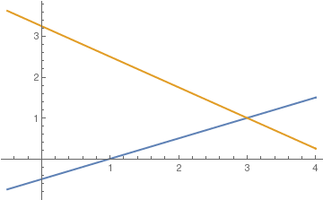
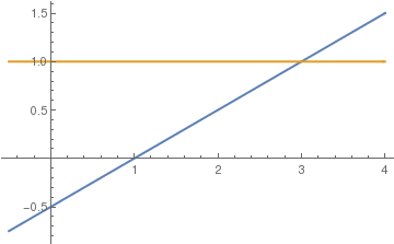
The last equation 10y = 10 reveals y = 1, and we go up the
triangle to x = 3. This quick process is called
back substitution. It is used for upper triangular systems of any size,
after forward elimination is complete. We plot our equations with
Mathematica.
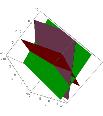
Two lines after eliminating variable y.
Which variable should you eliminate, x or y? For a computer, it does not matter, but for humans it does because it is more attractive. So mostly for educational purposes, we will follow tradition and we will eliminate variables from left to right in order to reduce the matrices into upper triangular form.
However, remember that when you write codes for practical calculations, it does not matter which variable you
eliminate and in what order---computer does not care!
When we used matrix form corresponding to the given system of equations, we
marked with red color special positions in the corresponding augmented matrix
because they important for understanding. These positions are usually referred to as pivots.
■
End of Example 1
Example 2:
Now we consider slightly different
system of algebraic equations
\begin{align*}
x -2\, y &= 1 , \\
3\,x - 6\,y &= 13 .
\end{align*}
Eliminating variable x by subtracting 3 times first equation from the
second one, we obtain
<
\begin{align*}
x -2\, y &= 1 , \\
0\,x - 0\,y &= \color{red}{10} .
\end{align*}
There is no solution. Remember that zero is never allowed as a pivot, hence
we get an equation with a pivot at the last column.
The last line in the matrix shows that every x and y satisfy the
equation 0·x + 0·y = 0. There is really only one
equation x - 2y = 1. One of the variables is free when another
one is expressed through the free one:
\[
x = 1 + 2\,y \qquad \mbox{or} \qquad y = \left( x-1 \right) /2 ,
\]
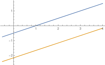
when y or x is freely chosen, respectively. There is no need to
plot one straight line that includes both equations because every its point
satisfies both equations. We have a whole line of solutions.
■
End of Example 3
Example 4:
Consider the system of algebraic equations
For this system, we cannot choose the first coefficient as a pivot because by
definition pivot cannot be a zero. So exchange two equations to obtain an
equivalent augmented matrix:
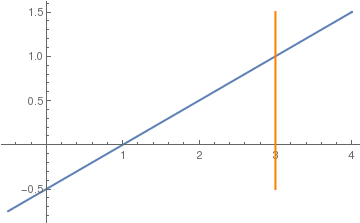
The new system is already triangular, so one of the lines is parallel to an
axis.
■
End of Example 4
To understand Gaussian elimination, you have to go beyond 2×2 systems of
equations. Therefore, we present examples of 3×3 systems of equations that will
be enough to see the pattern. Other example with rectangular matrices to
follow.
Example 5:
Consider the system of algebraic equations
This matrix contains all of the information in the system of equations without
the unknown variables x, y, and z to carry around. Now
we perform the process of elimination. The notation to the right of each
matrix describes the row operations that were performed to get the matrix on
that line. For example 2R1+R2 ↦ R2 means
"replace row 2 with the sum of 2 times row 1 and row 2."
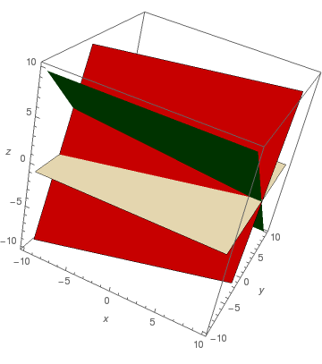
Planes in the echelon form.
We can now easily solve for x, y, and z by
back-substitution to obtain x = 1, y = -2, and
z = -1.
For a system of equations with a 3x3 matrix of coefficients, the goal of the process of Gaussian Elimination
is to create (at least) a triangle of zeroes in the lower left hand corner of the matrix below the diagonal.
Note that you may switch the order of the rows at any time in trying to get to this form.
a1 = ContourPlot3D[x - 3 y + z == 6,
{x, -10, 10}, {y, -10, 10}, {z, -10, 10},
AxesLabel -> {x, y, z}, Mesh -> None, ContourStyle -> Directive[Red]];
f2[x_, y_] := (-2* x + y-1)/5;
a2 = ParametricPlot3D[{x, y, f2[x, y]},
{x, -10, 10}, {y, -10, 10},
AxesLabel -> {x, y, z}, Mesh -> None, PlotStyle -> Directive[Green]];
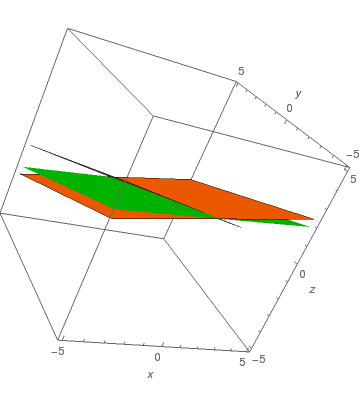
No solution.
We keep x in the first equation and eliminate it from the other
equations. To do so, add -1 times equation 1 to equation 2. After some
practice, this type of calculation is usually performed mentally. However,
it is convenient to use software:
Notice the last equation reads: 0=5. This is not possible. So the system has
no solutions; it is not possible to find values x, y, and
z that satisfy all three equations simultaneously.
■
End of Example 6
Example 7:
Consider the system of algebraic equations
Notice the last equation: 0=0 (this resulted from equation 3 being a linear
combination of the other two equations). This is always true. And, we can
solve the first two equations to get x and y as functions of
z alone. Solving these equations, we get
To eliminate x1 from the last three equations, we multiply
the first equation by -1, -2, and 3, respectively. By adding the results to
the corresponding rows, it will introduce zeroes into positions below the pivot
(which we mark with red) in the first column:
Finally, multiplying the third row by 8 and adding to the last row, we obtain,
what is usually called the row echelon form for the given augmented matrix:
Example 9:
This example illustrates how we can use linear systems to determine how many molecules of various chemical compounds are required
as input to a chemical reaction, as well as how many molecules of different
compounds are produced as output.
When ethane (C₂H₆) burns in the presence of oxygen gas (O₂), it produces carbon dioxide (CO₂) and water vapor (H₂O). We thus say that the
“unbalanced” equation for burning ethane is
\[
C_2 H_6 + O_2 \, \to \, C\,O_2 + H_2 O .
\]
Since we don't know how many copies of each molecule are involved in
the reaction, we multiply each molecule by unknown (integer) coefficient and make a chemical equation
\[
x\,C_2 H_6 + y\,O_2 \, = \, z\,C\,O_2 + w\,H_2 O ,
\]
where integers x, y, z, and w represent how many copies of each molecule are present in
the reaction. Hence, each side of the equation above
has the same amount of each element on the left- and right-hand sides.
On the left-hand side of this chemical equation, we have 2y atoms of
oxygen (O) and on the right-hand side we have 2z + w atoms of oxygen, so we require
\[
2\,y = 2\, z + w \qquad \iff \qquad 2\,y - 2\, z - w =0 .
\]
Similarly matching up the number of atoms of carbon (C) and hydrogen
(H) on the left- and right-hand sides reveals that
\[
2\,x = z \qquad\mbox{and} \qquad 6\,x = 2\,w .
\]
We thus have a linear system with 4 variables and 3 equations, which
we can solve with the aid of Mathematica. Since the number of equations is less than the number of unknowns, we choose one variable, say W as a free one.
Solve[{2*y== 2*z+w, 2*x==z, 6*x ==2*w}, {x,y,z}]
{{x -> w/3, y -> (7 w)/6, z -> (2 w)/3}}
Since one variable w is free, we could choose it so that all of the variables end up having integer values.
In particular, if we choose w = 6, then we getx = 2, y = 7, and z = 4, so that the balanced chemical equation becomes
\[
2\,C_2 H_6 + 7\,O_2 \, = \, 4\,C\,O_2 + 6\,H_2 O .
\]
■
End of Example 9
Chiò’s Method
Historically, before computers were available, most of examples and exercises in textbooks on Linear Algebra involved integers rather than fractions or irrational numbers or their floating point representations. Obviously, people
prefer to keep it that way avoiding heavy manual calculations. Inspired by Gaussian elimination algorithm, Felice Chiò proposed in 1853 a technique for determinant evaluation suitable for matrices with integer entries.
Felice (Félix) Chiò (1813–1871) was an Italian mathematician.
In Italian, his surname is spelled Chiò with a grave accent on the "ò".
This is confirmed by Italian academic sources and historical records.
However, some references use Chiò with an acute accent (é-style).
This is likely a typographical or transliteration inconsistency, possibly influenced by Spanish or French conventions.
In 1853, Felice (Félix) Chiò published his short Mémoire sur les fonctions connues sous le noms De Résultantes Ou De Déterminans.
The details of Chiò’s life are not well known. In 1846 when he was teaching mathemat- ics at the Military Academy of Turin, he presented a paper to the Academy of Sciences in Paris that was reported in its proceedings, Comptes Rendus (v. XXIII, no. 10, 7 September 1846), and published in 1853 in the form of two memoirs as Recherches sur la série de Lagrange. In 1854 he was appointed to the chair of physics ‘sublime’ at the Military Academy. In the same year he was appointed professor of mathematical physics at the University of Turin.
We demonstrate his approach, which is referred to as Chiò’s method, in some examples.
Let us consider a 3 × 3 matrix
\[
{\bf A} = \begin{bmatrix} 2& \phantom{-}3& -1 \\ 3& -2& \phantom{-}4 \\ 1& \phantom{-}5& \phantom{-}2 \end{bmatrix} .
\]
Suppose we want to treat the first entry in the first row as a pivot. In order to eliminate all entries in the first column below the pivot, we multiply by it (in our case, by "2") other rows:
\[
{\bf A}_1 = \begin{bmatrix} \fbox{2}& \phantom{-}3& -1 \\ 6& -4& \phantom{-}8 \\ 2& 10& \phantom{-}4 \end{bmatrix} .
\]
A = {{2, 3, -1}, {3, -2, 4}, {1, 5, 2}};
With row reductions R₂ ← R₂ − 3·R₁ and R₃ ← R₃ − R₁, we obtain an equivalent matrix
\[
{\bf A}_2 = \begin{bmatrix} \fbox{2}& \phantom{-}3& -1 \\ 0& -13& 11 \\ 0& \phantom{-}7& \phantom{-}5 \end{bmatrix} .
\]
Multiplying the second row by 7 and adding to the third row, we get
A4 = {A3[[1]], A3[[2]], A3[[3]] + 7*A3[[2]]}
{{2, 3, -1}, {0, -13, 11}, {0, 0, 142}}
\[
{\bf A}_4 = \begin{bmatrix} 2& 3& -1 \\ 0& \fbox{-13}& 11 \\ 0& 0& 142 \end{bmatrix} .
\]
This all-integer approach is easier for mental calculations.
This treatment of Chiò's technique is simplified by the assumption that all except perhaps the last
few of the leading principal submatrices of A are invertible. This simplification is tantamount to
the application in advance of whatever row and/or column exchanges would otherwise be found
during Chiò’s elimination process to be necessary to ensure the assumption’s validity; this is not
a significant restriction so far as matrix computations are concerned. However, this restriction
does prevent our treatment of Chiò’s trick from being applied directly to explain how a similar
trick works during the computations of greatest common divisors of pairs of polynomials, and the
computations of continued fraction expansions of rational functions.
Chiò’s algorithm defines a sequence of matrices A(k) with elements 𝑎(k)i,j:
𝑎(0)₀,₀ := 1
A(1) : = A ;   so 𝑎(1)i,j = 𝑎i,j
for k = 1, 2, 3, … in turn,
    𝑎(k+1)i,j := (𝑎(k)k,k · 𝑎(k)i,j − 𝑎(k)i,k · 𝑎(k)k,j) / 𝑎(k-1)k-1,k-1
     for all i > k and j > k
Of course, the algorithm would fail if any 𝑎(k-1)k-1,k-1 = 0, which is impossible due to our simplification assumption.
Example 10:
Using Mathematica, we generate a 4-by-4 matrix