
Introduction to Linear Algebra
Systems of Linear Equations
- Introduction
- Linear systems
- Vectors
- Linear combinations
- Matrices
- Planes in ℝ³
- Equation A x = b
- Sensitivity of solutions
- Linear independence
- Plane transformations
- Space transformations
- Linear transformations
- Affine maps
- Exercises
- Answers
Matrix Algebra
- Introduction
- Manipulation of matrices
- Partitioned matrices
- Block matrices
- Matrix operators
- Determinants
- Cofactors
- Cramer's rule
- Chiò's method
- Equivalent matrices
- Elimination: A = L U
- PLU factorization
- Reflection
- Givens rotation
- Special matrices
- Exercises
- Answers
Vector Spaces
- Introduction
- Motivation
- Vector spaces
- Bases
- Dimension
- Coordinate systems
- Linear transformations
- Change of basis
- Matrix transformations
- Compositions
- Isomorphisms
- Dual transformations
- Quotient spaces
- Wedge products
- Rotors
Eigenvalues, Eigenvectors
- Introduction
- Characteristic polynomials
- Companion matrix
- Algebraic and geometric multiplicities
- Minimal polynomials
- Eigenspaces
- Where are eigenvalues?
- Eigenvalues of A B and B A
- Generalized eigenvectors
- Similarity
- Diagonalizability
- Self-adjoint operators
- Exercises
- Answers
Euclidean Spaces
- Introduction
- Euclidean space
- Bilinear transformations
- Norm and distance
- Matrix norms
- Dual norms
- Dual transformations
- Examples of transformations
- Orthogonality
- Gram--Schmidt Process
- Orthogonal matrices
- Self-adjoint matrices
- Unitary matrices
- Projection operators
- QR-decomposition
- Least Square Approximation
- Quadratic forms
- Exercises
- Answers
Canonical forms
- Introduction
- 2D decomposition
- 3D decomposition
- Symmetric matrices
- Symmetric matrices
- Pseudoinverse
- URV-decomposition
- LU-decomposition
- QR-decomposition
- Cholesky decomposition
- Schur decomposition
- Positive matrices
- Roots
- Polar factorization
- Spectral decomposition
- CUR decomposition
- Exercises
- Answers
Applications
- Introduction
- Circles along curves
- TNB frames
- GPS problem
- Poisson equation
- Graph theory
- Error correcting codes
- Electric circuits
- FSA
- Markov chains
- Cryptography
- Wave-length transfer matrix
- Computer graphics
- Linear Programming
- Hill's determinant
- Fibonacci matrices
- Discrete dynamic systems
- Discrete Fourier transform
- Fast Fourier transform
- Curve fitting
- Answers
Miscellany
- Introduction
- Circles along curves
- TNB frames
- Differential forms
- Calculus
- Vector representations
- Matrix representations
- Change of basis
- Orthonormal Diagonalization
- Generalized inverse
- Differential forms
Preliminaries
- Complex Number Operations
- Sets
- Polynomials
- Polynomials and Matrices
- Computer solves Systems of Linear Equations
- Location of Eigenvalues
- Power Method
- Iterative Method
- Similarity and Diagonalization
Glossary
Reference

This Book is licensed under Creative Commons Attribution-NonCommercial-NoDerivs 3.0 Unported License
The Wolfram Mathematic notebook which contains the code that produces all the Mathematica output in this web page may be downloaded at this link. Caution: This notebook will evaluate, cell-by-cell, sequentially, from top to bottom. However, due to re-use of variable names in later evaluations, once subsequent code is evaluated prior code may not render properly. Returning to and re-evaluating the first Clear[ ] expression above the expression no longer working and evaluating from that point through to the expression solves this problem.
Remove[ "Global`*"] // Quiet (* remove all variables *)
This section is divided into a number of subsections, links to which are:
Every linear transformation T : 𝔽n ⇾ 𝔽n can be uniquely (subject to utilizing standard basis) associated with a square matrix ⟦T⟧ ∈ 𝔽n×n and vice versa. This one-to-one correspondence between linear transformations and square matrices allows us to identify every transformation with a matrix that acts on vectors upon multiplication. Therefore, analysis of matrices is the same as dealing with linear transformations. Out of many matrices/transformations there is a very important class consisting of invertible matrices.
In what follows, we consider rotations as elements of an orthogonal group under field ℝ of real numbers. Matrices that correspond to positive (= counterclockwise) rotation operations provide a very valuable example of special class of matrices. The most general three-dimensional rotation matrix represents a counterclockwise rotation by an angle θ about a fixed axis that lies along the unit vector n, also usually denoted by \( \displaystyle \hat{\bf n} = (n_x , n_y , n_z ). \)
True
Det[A]
% // FullSimplify
-1
Det[A]
% // FullSimplify
1
Rotations
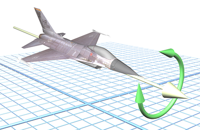
An in-depth study of rotations can become a lifelong project so we restrict ourselves to rotations in ℝ² and ℝ³. Unlike two dimensional case, rotations do not commute. For instance, Ry(45°)∘Rx(90°) ≠ Rx(90°)∘Ry(45°), where Rx(θ) is rotation around the x-axis by θ in ℝ³. (As usual, B∘A means the composition of action A followed by action B.) By a rotation, we always mean a linear transformation in either ℝ² or ℝ³.Any 3D isometry with a fixed point O has an invariant plane and an invariant axis which intersect at right angle at O. It is a customary to define rotation to be positive if rotation occurs in counterclockwise direction. An orientation–preserving isometry with fixed point O is a 3D rotation through a certain angle around its invariant axis in its invariant plane.
The previous example shows that rotations on ℝ² are commutative. We treat the identity matrix as a rotation through 0 radians. With that, we can say that the rotations on ℝ² are the mappings in O₂(ℝ) with determinant 1. Since det(A B) = detA detB for matrices A and B when the product A B is defined, and since det(A−1) = 1/det(A) when det(A) ≠ 0, we see that the rotations on ℝ² form a subgroup of O₂(ℝ). That subgroup is denoted SO₂(ℝ) and is called the special orthogonal group on ℝ².
In general, the orthogonal group in dimension n has two connected components. The one that contains the identity element is a normal subgroup, called the special orthogonal group, and denoted SO₂(ℝ) or SO(n). It consists of all orthogonal matrices of determinant 1. This group is also called the rotation group, generalizing the fact that in dimensions 2 and 3, its elements are the usual rotations around a point (in dimension 2) or a line (in dimension 3). In low dimensions, these groups have been widely studied. The other component consists of all orthogonal matrices of determinant −1. This component does not form a group, as the product of any two of its elements is of determinant 1, and therefore not an element of the component.
Let α be the angle between x and y and let β denote the angle between Ax and Ay. Using Ax • Ay = x • y again, we get |Ax||Ay| cos(β) = Ax • Ay = x • y = |x||y| cos(α). Because |Ax| = |x|, |Ay| = |y|, this means cos(α) = cos(β). As we have defined the angle between two vectors to be a number in [0, π] and cos is monotonic on this interval, it follows that α = β.
To the converse: if A preserves angles and length, then v1 = Ae₁, … , vn = Aen form an orthonormal basis. By looking at B = ATA this shows the off-diagonal entries of B are 0 and diagonal entries of B are 1. The matrix A is orthogonal.
Here is how Mathematica constructs a larger matrix from smaller "block" matrices
\( \displaystyle \quad a = - \sqrt{1 - c^2} \quad |\, | \ a = \sqrt{1-c^2} \)
\( \displaystyle \quad b= - \sqrt{1 - d^2} \quad |\, | \ b = \sqrt{1-d^2} \)
Numeric Example
Rotation Matrices
The effect of rotating a vector by θ is the same as the effect obtained by rotation of the frame of reference. When point O on the axis of rotation is chosen, it can be used to define a frame (e₁, e₂, e₃). Let (u₁, u₂, u₃) be the image of the frame under a transformation (rotation in our case). We write every vector ui, i = 1, 2, 3, in coordinates of the original frame:
Mathematica has its own command for rotation matrices. For instance,
The simplest such representation is based on Euler’s theorem, stating that every rotation can be described by an axis of rotation and an angle around it. A compact representation of axis and angle is a three-dimensional rotation vector whose direction is the axis and whose magnitude is the angle in radians. The axis is oriented so that the acute-angle rotation is counterclockwise around it. As a consequence, the angle of rotation is always nonnegative, and at most π.
Translation and rotation are the only rigid body transformations. Recall that a rigid body transformation is one that changes the location and orientation of an object, but not its shape. All angles, lengths, areas, and volumes are preserved by rigid body transformations. All rigid body transformations are orthogonal, angle-preserving, invertible, and affine.
Suppose that quadratic equation \[ \chi_M (\lambda )/(\lambda -1) = 0 \] has two real roots of magnitude 1. Then we have two options for eigenvalues of matrix M to be either (1, 1, 1) or (1, −1, −1). If the equation above has complex roots, then for its value of z and complex conjugate z*, we have \[ \chi_M (\lambda ) = \det (\lambda {\bf I} - {\bf M} ) = \left(\lambda -1 \right) \cdot \left( \lambda - z \right) \cdot \left( \lambda - z^{\ast} \right) . \] To the pair of complex eigenvalues corresponds the eigenspace which is perpendicular to the axis of rotation. Matrix M acts on these eigenvectors as a rotation.
From Euler's rotating theorem (see section), it follows that every spacial rotation in ℝ³ has a rotation axis, which we identify with a unit vector along the line of rotation \( \displaystyle \quad \hat{\bf n} = (n_x , n_y , n_z ). \quad \) Let O be the origin in regular Euclidean space ℝ³ and let θ denote the angle of rotation.We denote by rot(n, θ) the corresponding around axis identified with unit vector n by angle θ.
- rot(−n, −θ) = rot(n, θ).
- rot(n, θ + 2kπ) = rot(n, θ) for any integer k.
- the angle θ can be restricted to θ ∈ [0, π]; this angle may be discontinuous at end points,
- when θ = 0, the rotation is undetermined.
Fixed Points of Rotation Matrices
For a rotation matrix (or operator) R, a fixed point equation R v = v is actually an eigenvector equation meaning that λ = 1 is an eigenvalue of the rotation matrix. Since det(R) = 1, the rotation matrix in ℝ³ has two other complex conjugate eigenvalues exp(±jϕ), where j is the unit imaginary vector in complex plane ℂ, so j² = −1. The eigenvector of unit length, designated n, defines an axis of rotation. Every vector on this axis is a fixed point for matrix operator R so they are left unchanged by the displacement. The eigenvectors corresponding to the the complex conjugate pair span the plane normal to the axis of rotation.
There exists a basis in ℝ³ so that a rotation matrix has the form
By Euler’s theorem, any rotation matrix R is fully defined by the pair (ϕ, n), where ϕ ∈ [0, 2 π] is the angle of rotation about the axis with respect to the initial configuration. Since 2 scalar parameters are needed to represent a unit vector in ℝ³, Euler’s theorem implies that a generic rotation tensor can be described with no less than 3 scalar parameters (1 for the rotation angle and 2 for the unit vector along the axis), i.e., the dimension of the manifold of the rotation group SO(3). Any description of rotation employing a set made by 3 scalar parameters is termed minimal, while it is referred as m-redundant when the set employs (3 + m) parameters. In the latter case, m scalar constraints must be enforced to ensure that the parameter set indeed corresponds to an element of SO(3).
In kinematics, Mozzi-Chasles’ fundamental theorem on rigid motion states: “any rigid motion may be represented by a planar rotation about a suitable axis, followed by a uniform translation along that same axis”. The proof that a spatial displacement can be decomposed into a rotation and slide around and along a line is attributed to the astronomer and mathematician Giulio Mozzi (1763), in fact the screw axis is traditionally called asse di Mozzi in Italy. However, most textbooks refer to a subsequent similar work by Michel Chasles dating from 1830.
Mozzi-Chasles’ theorem entails that a generic rigid displacement can be described with no less than 6 scalar parameters (3 for the rotation, 2 for the position of unit vector a, and 1 for the scalar translation), i.e. the dimension of the manifold of the euclidean group SE(&Epf;³). As for rotation, any description of motion employing 6 parameters is termed minimal, while it is referred as redundant when employing more than 6 parameters.
Orientation in 3D
Although orientation is closely related to direction, but it is not exactly the same. The fundamental difference between direction and orientation is seen conceptually by the fact that we can parameterize a direction in 3D with just two numbers (the spherical coordinate angles), whereas an orientation requires a minimum of three numbers. For example, a vector has a direction, but not an orientation---it can be twisted without changing its length and direction.
Typically, the orientation is given relative to a frame of reference, usually specified by a Cartesian coordinate system. Two objects sharing the same direction are said to be codirectional (as in parallel lines). Two directions are said to be opposite if they are the additive inverse of one another, as in an arbitrary unit vector and its multiplication by −1. Two directions are obtuse if they form an obtuse angle (greater than a right angle) or, equivalently, if their scalar product or scalar projection is negative.
Orientation cannot be described in absolute terms---you need to chose a frame first. Then an orientation is given by a rotation from some known reference orientation (often called the “identity” or “home” orientation). An example of an orientation is, “Standing upright and facing east.” The amount of rotation is known as an angular displacement. In other words, describing an orientation is mathematically equivalent to describing an angular displacement. You might also hear the word “attitude” used to refer the orientation of an object, especially if that object is an aircraft.
- Show that GLn(𝔽) is not a vector space.
- Let \[ \mathbf{A} = \begin{bmatrix} \cos\theta & \sin\theta \\ \sin\theta & -\cos\theta \end{bmatrix} , \quad \mathbf{v} = \begin{bmatrix} 1 + \cos\theta \\ \sin\theta \end{bmatrix} , \quad \mathbf{x} = \begin{bmatrix} \sin\theta \\ 1 - \cos\theta \end{bmatrix} . \] Show that A v is a scalar multiple of v and that A x is a scalar multiple of x.
- Which of the following matrices is orthogonal? \[ ({\bf a})\quad \begin{bmatrix} 1&1&1&1 \\ 1&-1&1&-1 \\ 1&1&-1&-1 \\ 1&-1&-1&1 \end{bmatrix} , \qquad ({\bf b})\quad \begin{bmatrix} 0&0&1&0 \\ 0&-1&0&0 \\ -1&0&0&0 \\ 0&0&0&1 \end{bmatrix} , \] \[ ({\bf c})\quad \begin{bmatrix} 1&0&0 \\ 0&-1&1 \\ 0&0&-1 \end{bmatrix} , \qquad ({\bf d})\quad \begin{bmatrix} \cos (3) & -\sin (3) &0&0 \\ \sin (3) & \cos (3) &0&0 \\ 0&0& \cos (1) &\sin (1) \\ 0&0&\sin (1) & -\cos (1) \end{bmatrix} , \]
- For any real numbers p, q, r, and s, matrices of the form \( \displaystyle \quad \begin{bmatrix} p&-q&-r&-s \\ q&p&s&-r \\ r&-s&p&q \\ s&r&-q&p \end{bmatrix} . \quad \) are called quaternions. Find a basis for the set of quaternion matrices.
- Anton, Howard (2005), Elementary Linear Algebra (Applications Version) (9th ed.), Wiley International
- Dunn, F. and Parberry, I. (2002). 3D math primer for graphics and game development. Plano, Tex.: Wordware Pub.
- Foley, James D.; van Dam, Andries; Feiner, Steven K.; Hughes, John F. (1991), Computer Graphics: Principles and Practice (2nd ed.), Reading: Addison-Wesley, ISBN 0-201-12110-7
- Matrices and Linear Transformations
- Rogers, D.F., Adams, J. A., Mathematical Elements for Computer Graphics, McGraw-Hill Science/Engineering/Math, 1989.
- Shuster, M. D., A survey of attitude representations, Journal of the Astronautical Sciences 41(4) 439–517 (1993).
- Watt, A., 3D Computer Graphics, Addison-Wesley; 3rd edition, 1999.