
Introduction to Linear Algebra
Systems of Linear Equations
- Introduction
- Linear systems
- Vectors
- Linear combinations
- Matrices
- Planes in ℝ³
- Equation A x = b
- Sensitivity of solutions
- Linear independence
- Plane transformations
- Space transformations
- Linear transformations
- Affine maps
- Exercises
- Answers
Matrix Algebra
- Introduction
- Manipulation of matrices
- Partitioned matrices
- Block matrices
- Matrix operators
- Determinants
- Cofactors
- Cramer's rule
- Chiò's method
- Equivalent matrices
- Elimination: A = L U
- PLU factorization
- Reflection
- Givens rotation
- Special matrices
- Exercises
- Answers
Vector Spaces
- Introduction
- Motivation
- Vector spaces
- Bases
- Dimension
- Coordinate systems
- Linear transformations
- Change of basis
- Matrix transformations
- Compositions
- Isomorphisms
- Dual transformations
- Quotient spaces
- Wedge products
- Rotors
Eigenvalues, Eigenvectors
- Introduction
- Characteristic polynomials
- Companion matrix
- Algebraic and geometric multiplicities
- Minimal polynomials
- Eigenspaces
- Where are eigenvalues?
- Eigenvalues of A B and B A
- Generalized eigenvectors
- Similarity
- Diagonalizability
- Self-adjoint operators
- Exercises
- Answers
Euclidean Spaces
- Introduction
- Euclidean space
- Bilinear transformations
- Norm and distance
- Matrix norms
- Dual norms
- Dual transformations
- Examples of transformations
- Orthogonality
- Gram--Schmidt Process
- Orthogonal matrices
- Self-adjoint matrices
- Unitary matrices
- Projection operators
- QR-decomposition
- Least Square Approximation
- Quadratic forms
- Exercises
- Answers
Canonical forms
- Introduction
- 2D decomposition
- 3D decomposition
- Projectors
- Direct-sum decompositions
- Cyclic decompositions
- Symmetric matrices
- Symmetric matrices
- Pseudoinverse
- URV-decomposition
- LU-decomposition
- QR-decomposition
- Cholesky decomposition
- Schur decomposition
- Positive matrices
- Roots
- Polar factorization
- Spectral decomposition
- CUR decomposition
- Exercises
- Answers
Applications
- Introduction
- Circles along curves
- TNB frames
- GPS problem
- Coriolis acceleration
- Poisson equation
- Graph theory
- Error correcting codes
- Electric circuits
- FSA
- Markov chains
- Cryptography
- Wave-length transfer matrix
- Computer graphics
- Linear Programming
- Hill's determinant
- Fibonacci matrices
- Discrete dynamic systems
- Discrete Fourier transform
- Fast Fourier transform
- Curve fitting
- Answers
Miscellany
- Introduction
- Circles along curves
- TNB frames
- Differential forms
- Calculus
- Vector representations
- Matrix representations
- Change of basis
- Orthonormal Diagonalization
- Generalized inverse
- Differential forms
Preliminaries
- Complex Number Operations
- Sets
- Polynomials
- Polynomials and Matrices
- Computer solves Systems of Linear Equations
- Location of Eigenvalues
- Power Method
- Iterative Method
- Similarity and Diagonalization
Glossary
Reference

This Book is licensed under Creative Commons Attribution-NonCommercial-NoDerivs 3.0 Unported License
There are two reasons to use the sum of two vector spaces. One of them is the way to build new vector spaces from old ones. Another reason is to decompose the known vector space into sum of two (smaller) spaces. Since we consider linear transformations between vector spaces, these sums lead to representations of these linear maps and corresponding matrices into forms that reflect these sums. In many very important situations, we start with a vector space V and can identify subspaces “internally” from which the whole space V can be built up using the construction of sums. However, the most fruitful results we obtain for a special sum, called the direct sum.
Products and Sums
There is a strong connection between products and suns of vector spaces. Before exploring the topic. let us remind some information that is related to this section. For any two sets A and B, their Cartesian product consists of all ordered pairs (𝑎, b) such that 𝑎 ∈ A and b ∈ B,Let A and B be nonempty subsets of a vector space V. The sum of A and B, denoted A + B, is the set of all possible sums of elements from both subsets: \( A+B = \left\{ a+b \, : \, a\in A, \ b\in B \right\} = \mbox{span}(A \cup B) . \)
This definition is naturally extended on finite number of subsets X₁, X₂, … , Xn of vector space V. Now we go to our main topic, sums of subspaces.Sums of Subspaces
Now to prove that W₁ + W₂ + ⋯ + Wn is the smallest subspace containing W₁, W₂, … , Wn, we will show that any subspace of V containing W₁, W₂, … , Wn contains the sum W₁ + W₂ + ⋯ + Wn.
Let W be any subspace containing W₁, W₂, … , Wn. Let w = w₁ + w₂ + ċ + wn ∈ WW₁ + W₂ + ⋯ + Wn, where wi ∈ Wi for all i = 1, 2, … , n. Since W is a subspace of V and W contains the sum W₁ + W₂ + ⋯ + Wn, w ∈ W.
 |
 |
Any vector . (x, y) ∈ ℝ² can be written as a linear combination of elements of W₁ and . W₂ as follows: \[ \mathbb{R}^2 \ni (x, y) = \left( \frac{x+ 2\,y}{2} , \ \frac{x + 2\,y}{4} \right) + \left( \frac{x - 2\,y}{2} , \ \frac{2\,y -x}{4} \right) \in W_1 + W_2 . \] As W₁ + W₂ is a two-dimensional subspace of ℝ², this implies that W₁ + W₂ = Ropf;². Also observe that the representation of any vector as the sum of elements in W₁ and W₂ is unique here. ■
In 1945, P.H. Leslie published the paper on how matrices could be used to predict the evolution of populations. Patrick Holt Leslie (1900---1972) nickname "George" was a Scottish physiologist best known for his contributions to population dynamics, including the development of the Leslie matrix, a mathematical tool widely used in ecological and demographic studies.
The Leslie matrix model requires that the interval between consecutive observations have the same length as each age group. Let \[ {\bf n}(0) = \begin{pmatrix} n_ (0) \\ n_2 (0) \\ \vdots \\ n_m (0) \end{pmatrix} \] be the initial age distribution vector displaying the number of humans in each age group at time t₀ = 0 and let n(tk) be the number of people in each group at time tk, i.e., the age distribution vector at time tk.
During a 5-year time span, it is expected to have deaths, births and aging in each age group. Hence, for i = 1, 2, … n, let bi denote the expected number of humans born to the age group i between the times tk and tk+1, and let sis be the proportion of people in the group i at time tk that are expected to be in the group i+1 at time tk+1.
It follows that \[ n_1 (t_{k+1}) = n_1 (t_k )\,b_1 + n_2 (t_k )\,b_2 + \cdots + n_m (t_k )\,b_m , \] and for i = 2, 3, … , \[ n_i (t_{k+1}) = s_{i-1}n_{i-1} (t_k ). \] This leads to the Leslie matrix models \[ \mathbf{L} = \begin{bmatrix} b_1 & b_2 &b_3& \cdots & b_m \\ s_1 &0&0& \cdots & 0 \\ 0& s_2 & 0 & \cdots & 0 \\ \vdots & \vdots & \vdots & \ddots & \vdots \\ 0&0& \cdots & s_{m-1}&0 \end{bmatrix} . \] Now we can rewrite the Lesley equation in succinct matrix/vector form \[ {\bf n}(t_{k+1}) = \mathbf{L}\,\mathbf{n}(t_k ) \] and, in general, we have for k = 0, 1, 2, … , \[ {\bf n}(t_{k+1}) = \mathbf{L}^k \mathbf{n}(0) . \] ■
Direct Sums
Let α be a set of generators (meaning that span(α) = A) of subspace A ⊂ V and β be a set of generators of subspace B ⊂ V. Their union α ∪ β generates the sum, A + B. If x ∈ A, y ∈ B, and w ∈ A ∩ B, then
Now we come to a particular but very important case of sums of subspaces when every vector from a vector space V can be uniquely decomposed into sum of vectors from given subspaces.
A vector space V is called the direct sum of V₁ and V₂ if V₁ and V₂ are subspaces of V such that \( V_1 \cap V_2 = \{ 0 \} \) and \( V_1 + V_2 = V. \) This means that every vector v from V is uniquely represented via sum of two vectors \( {\bf v} = {\bf v}_1 + {\bf v}_2 , \quad {\bf v}_1 \in V_1 , \ {\bf v}_2 \in V_2 . \) We denote that V is the direct sum of V₁ and V₂ by writing \( V = V_1 \oplus V_2 . \)
The symbol ⊕, which is a plus sign inside a circle, serves as a reminder that we are dealing with a special type of sum of subspaces— each element in the direct sum can be represented only one way as a sum of elements from the specified subspaces.
For n = 2, the meaning of independence is zero intersection, i.e., X₁ and X₂ are independent if and only if X₁ ∩ X₂ = {0}. If n > 2, the independence of subspaces X₁, X₂, … , Xn says much more than X₁ ∩ X₂ ∩ ⋯ ∩ Xn = {0}. It means that each subspace Xi intersects the sum of the other subspaces only in the zero vector.
Since in vector spaces uniqueness expansion v = x₁ + x₂ + ⋯ + xn is equivalent to theindependence of subspaces, we can make the following
Observation: Let V be a finite-dimensional vector space, and let X₁, X₂, … , Xn be its subspaces. Then sum X = X₁ + X₂ + ⋯ + Xn is direct if and only is the subspaces X₁, X₂, … , Xn are independent.
Theorem 8: Suppose that V₁, V₂, … , Vn are subspaces of V. Define a linear map Γ : V₁ × V₂ × ⋯ × Vn → V₁ + V₂ + ⋯ _ Vn by \[ \Gamma \left(\mathbf{v}_1 , \mathbf{v}_2 , \ldots , \mathbf{v}_n \right) = \mathbf{v}_1 + \mathbf{v}_2 + \cdots + \mathbf{v}_n . \] Then V₁ + V₂ + ⋯ _ Vn is a direct sum if and only if Γ is injective.
Also any 2-by-2 matrix from V can be expressed as a sum of elements in W₁ and W₂. However, this expression is not unique. For example, \[ \begin{bmatrix} 3&4 \\ 1& 2 \end{bmatrix} = \begin{bmatrix} 3&4 \\ 0& 2 \end{bmatrix} + \begin{bmatrix} 0&0 \\ 1&0 \end{bmatrix} \] and \[ \begin{bmatrix} 3&4 \\ 1& 2 \end{bmatrix} = \begin{bmatrix} 0&4 \\ 0&0 \end{bmatrix} + \begin{bmatrix} 3&0 \\ 1&2 \end{bmatrix} . \] ■
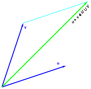
If we choose two arbitrary not parallel vectors u and v on the plane, then spans of these vectors generate two vectors spaces that we denote by U and V, respectively. Therefore, U and V are two lines containing vectores u and v, respectively. Their sum, \( U + V = \left\{ {\bf u} +{\bf v} \,: \ {\bf u} \in U, \ {\bf v} \in V \right\} \) is the whole plane \( \mathbb{R}^2 . \)
g2 = Graphics[{Blue, Thickness[0.01], Arrow[{{0, 0}, {1, 3}}]}]
g3 = Graphics[{Green, Thickness[0.01], Arrow[{{0, 0}, {4, 4}}]}]
g4 = Graphics[{Cyan, Thickness[0.005], Line[{{1, 3}, {4, 4}}]}]
g5 = Graphics[ Text[Style[
ToExpression["u + v \\notin U\\cup V", TeXForm, HoldForm],
FontSize -> 14, FontWeight -> "Bold", FontColor -> Black], {3.6, 3.5}, {0, 1}, {1, 1}]]
g6 = Graphics[
Text[StyleForm["u", FontSize -> 14, FontWeight -> "Bold",
FontColor -> Blue], {2.6, 1.2}, {0, 0.8}, {2.8, 1}]]
g7 = Graphics[
Text[StyleForm["v", FontSize -> 14, FontWeight -> "Bold",
FontColor -> Blue], {1.1, 2.8}]]
Show[g1, g2, g3, g4, g5, g6, g7]
Suppose we have a vector space V over field 𝔽 and subspaces W₁, W₂, … , Wn of V. Then it is not easy to check whether every element in V has a unique representation as the sum of elements of W₁, W₂, … , Wn. The following theorem provides a solution for this.
Theorem 2: Let V be a vector space over field 𝔽 and W₁, W₂, … , Wn be subspaces of V. Then V = = W₁ ⊕ W₂ ⊕ ⋯ ⊕ Wn if and only if the following conditions are satisfied:
- V = W₁ + W₂ + ⋯ + Wn;
- zero vector has only the trivial representation.
It is easy to see that any polynomial (or function) can be ubiquely decomposed into direct sum of even and odd counterparts:
Theorem 6: Let V be a finite-dimensional vector space over field . 𝔽 and V ₁, i>V ₂ be two subspaces of V, then \[ \dim \left( V_1 + V_2 \right) = \dim \left( V_1 \right) + \dim \left( V_2 \right) - \dim \left( V_1 \cap V_2 \right) . \]
Theorem 7: Let V be a finite-dimensional vector space over field 𝔽, and let V₁, V₂, … , Vn be subspaces of V such that V = V₁ + V₂ + ⋯ + Vn and . dim(V) = dim(V₁) + dim(V₂) + ⋯ + dim(Vn). Then V = V₁ ⊕ V₂ ⊕ ⋯ ⊕ Vn.
Now let 0 = v₁ + v₂ + ⋯ + vn, where vi ∈ Vi. Since βi is a basis for .Vi, each vi ∈ Vi can be expressed uniquely as a sum of elements in βi. i.e., 0 can be written as a linear combination of elements of β. As β is a basis for V, this implies that the coefficients are zero. That is, vi = 0 for all i = 1, 2, … , n. Therefore, V = V₁ ⊕ V₂ ⊕ ⋯ ⊕ Vn.
Annihilators and Direct Sums
Consider a direct sum decomposition of a vector space over field 𝔽:Theorem 4: Let V = S ⊕ T be a direct decomposition of a vector space V. The extension by 0 map is an isomorphism from T* to S⁰, and so \[ T^{\ast} \cong S^0 . \] If V is finite-dimensional, then \[ \dim\left( S^0 \right) = \mbox{codim}\left( S \right) = \dim \left( V/S \right) = \dim V - \dim S . \]
Theorem 5: A linear functional on the direct sum V = S ⊕ T can be written as a sum of a linear functional that annihilates S and a linear functional that annihilates T, that is, \[ \left( S \oplus T \right)^{\ast} = S^0 \oplus T^0 . \]
- Suppose \[ U = \left\{ (x, x, y, y) \in\Mathbb{F}^4 \quad : \quad x, y \in \mathbb{F} \right\} \] ind a subspace W of 𝔽4 such that 𝔽4 = V ⊕ W.
- Let \[ U = \left\{ \left( x, y, x+y , x-y , 3\,y \right) \in \mathbb{F}^5 \ : \quad x, y \in \mathbb{F} \right\} . \] Find a subspace W of 𝔽5 such that 𝔽5 = U ⊕ W.
- For any i, 1 ≤ i ≤ n, prove \[ V_1 + V_2 + \cdots + V_n = \left( V_1 + V_2 + \cdots + V_i \right) + \left( V_{i+1} + \cdots + V_n \right) . \]
- Suppose \[ U = \left\{ \left( x, y, x+y , x-y , 3\,y \right) \in \mathbb{F}^5 \ : \quad x, y \in \mathbb{F} \right\} . \] Find three subspaces W₁, W₂, W₃ of 𝔽5, none of which equals f0}, such that 𝔽5 = W₁ ⊕ W₂ ⊕ W₃. that
- Prove or give a counterexample: if V₁, V₂, W are subspaces of V such that \[ V = V_1 \oplus W \quad\mbox{and} \quad V = V_2 \oplus W , \] then V₁ = V₂.
- Suppose U is a subspace of vector space V. What is U + U ?
- Axier, S., Linear Algebra Done Right. Undergraduate Texts in Mathematics (3rd ed.). Springer. 2015, ISBN 978-3-319-11079-0.
- Beezer, R.A., A First Course in Linear Algebra, 2017.
- Dillon, M., Linear Algebra, Vector Spaces, and Linear Transformations, American Mathematical Society, Providence, RI, 2023.
- Halmos, Paul Richard (1974) [1958]. Finite-Dimensional Vector Spaces. Undergraduate Texts in Mathematics (2nd ed.). Springer. ISBN 0-387-90093-4.
- Leslie. P.H., On the use of matrices in certain population mathematics. Biometrika 33, pages 183–212, 1945.
- Roman, Steven (2005). Advanced Linear Algebra. Undergraduate Texts in Mathematics (2nd ed.). Springer. ISBN 0-387-24766-1.