
Introduction to Linear Algebra
Systems of Linear Equations
- Introduction
- Linear systems
- Vectors
- Linear combinations
- Matrices
- Planes in ℝ³
- Equation A x = b
- Sensitivity of solutions
- Linear independence
- Plane transformations
- Space transformations
- Linear transformations
- Affine maps
- Exercises
- Answers
Matrix Algebra
- Introduction
- Manipulation of matrices
- Partitioned matrices
- Block matrices
- Matrix operators
- Determinants
- Cofactors
- Cramer's rule
- Chiò's method
- Equivalent matrices
- Elimination: A = L U
- PLU factorization
- Reflection
- Givens rotation
- Special matrices
- Exercises
- Answers
Vector Spaces
- Introduction
- Motivation
- Vector spaces
- Bases
- Dimension
- Coordinate systems
- Linear transformations
- Change of basis
- Matrix transformations
- Compositions
- Isomorphisms
- Dual transformations
- Quotient spaces
- Rank
- Solving A x = b
- Exercises
- Answers
Eigenvalues, Eigenvectors
- Introduction
- Characteristic polynomials
- Companion matrix
- Algebraic and geometric multiplicities
- Minimal polynomials
- Eigenspaces
- Where are eigenvalues?
- Eigenvalues of A B and B A
- Generalized eigenvectors
- Similarity
- Diagonalizability
- Self-adjoint operators
- Exercises
- Answers
Euclidean Spaces
- Introduction
- Euclidean space
- Bilinear transformations
- Norm and distance
- Matrix norms
- Dual norms
- Dual transformations
- Examples of transformations
- Orthogonality
- Gram--Schmidt Process
- Orthogonal matrices
- Self-adjoint matrices
- Unitary matrices
- Projection operators
- QR-decomposition
- Least Square Approximation
- Quadratic forms
- Exercises
- Answers
Canonical forms
- Introduction
- 2D decomposition
- 3D decomposition
- Projectors
- Direct-sum decompositions
- Cyclic decompositions
- Symmetric matrices
- Pseudoinverse
- URV-decomposition
- LU-decomposition
- QR-decomposition
- Cholesky decomposition
- Schur decomposition
- Positive matrices
- Roots
- Polar factorization
- Spectral decomposition
- CUR decomposition
- Exercises
- Answers
Applications
- Introduction
- Circles along curves
- TNB frames
- GPS problem
- Coriolis acceleration
- Poisson equation
- Graph theory
- Error correcting codes
- Electric circuits
- FSA
- Markov chains
- Cryptography
- Wave-length transfer matrix
- Computer graphics
- Linear Programming
- Hill's determinant
- Fibonacci matrices
- Discrete dynamic systems
- Discrete Fourier transform
- Fast Fourier transform
- Curve fitting
- Answers
Miscellany
- Introduction
- Circles along curves
- TNB frames
- Differential forms
- Calculus
- Vector representations
- Matrix representations
- Change of basis
- Orthonormal Diagonalization
- Generalized inverse
- Differential forms
Preliminaries
- Complex Number Operations
- Sets
- Polynomials
- Polynomials and Matrices
- Computer solves Systems of Linear Equations
- Location of Eigenvalues
- Power Method
- Iterative Method
- Similarity and Diagonalization
Glossary
Reference

This Book is licensed under Creative Commons Attribution-NonCommercial-NoDerivs 3.0 Unported License
This section is divided into a number of subsections, links to which are:
Remove[ "Global`*"] // Quiet (* remove all variables *)
2D Rotations
A rotation on the plane (2D, for short) about the origin has only one parameter, the angle, which defines the amount of rotation. The standard convention found in most math books is to consider counterclockwise rotation positive and clockwise rotation negative. We can do rotation about the origin using matrix multiplication. A rotation matrix is a transformation performed by matrix multiplication on vectors that results in rotating of the vector by angle θ in counterclockwise direction. WE use matrices in bracket notation when they are considered as operators on column vectors and we embrace matrices in parentheses when they operate on row vectors from right.When rotation occurs about a fixed point other than the origin, use the following three step approach:
- Move fixed point to origin,
- Rotate,
- Move fixed point back.
Frame Rotation -- Points fixed
Let us consider a plane ℝ², which is the Cartesian product of two real number lines, ℝ × ℝ. Upon choosing two perpendicular lines with uniform grid, we obtain a coordinate system or a frame. Since a grid has a natural order, these two lines become axes and usually they are visualized with arrows. The point of intersection of these two lines is called the origin. The horizontal line, known as abscissa is usually labeled with x, and the vertical line pointed up is known as ordinate, we label it will letter y.Note that, these two axes are ordered in the plane such that a 90 degree counter-clockwise rotation about the origin transfers the positive x-axis into the positive ordinate. The origin represents the zero point on each coordinate axis and is designated by the ordered pair of real numbers (0, 0). A unit vector on abscissa is usually denoted by i = (1, 0) ) or e₁, and the unit vector on ordinate is denoted by j = (0, 1) or e₂.
We fix a point P(x₀, y₀) in the xy-plane, which is also identified by vector \( \displaystyle \quad {\bf r} = \overline{OP} = (x_0 , y_0 )\quad \) because point P and vector r have the same coordinates. We are going to determine new coordinates of point P when frame O(x, y) is rotated by angle θ in counterclockwise direction (which is considered to be positive). For simplicity, we drop subscripts of point/vector in further derivation. Let the coordinates of P in the new frame be (X, Y), which can be expresed through its previous coordinates (x, y).
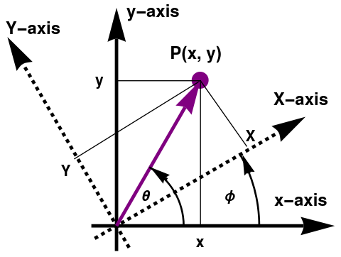
From Figure 1 we notice that the angle between the vector \( \displaystyle \quad {\bf r} = \overline{OP} \quad \) b>r and the rotated X-axis is θ − ϕ. Let r be the length of the vector r and ϕ be the angle between the vector and the positive x axis. Then, using ordinary right triangle trigonometry, we see that
If you are familiar with matrix multiplication (see Part 2 of this tutorial), we can replace a pair of equations with a concise formula. Wring coordinates as column vectors, we get
Point Rotation -- Frame fixed
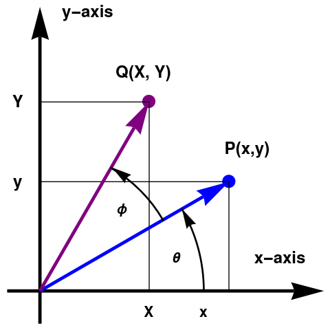
We begin with rotating a point P(x₀, y₀) in the xy-plane about the origin through an angle θ in counterclockwise direction. We demonstrate derivation of the rotation matrix in two ways. First, we use trigonometric relations, and then show that the same matrix can be obtained based on rotations of basic vectors i = (1, 0) and j = (0, 1),
Suppose that a given point P(x, y) is moved under rotation by angle ϕ into a new point Q(X, Y). In order to derive the rotation matrix, we recognize that the new point Q will be the same distance from the origin as the starting point P. So both points P and Q lie on the circle centered at the origin of radius r = |OP|. The point Q is just an extra angle ϕ, as measured from the positive abscissa (= x-axis) relative to the position of P at this circle. If the point P is at angle θ, then the new point Q is at the angle ϕ + θ. Since all the points on the circle of radius r with center at the origin can be written as \( \displaystyle r\,e^{{\bf j}\alpha} = \left( r\,\cos\alpha , r\,\sin\alpha \right) \) for some real number α. We know that point P has coordinates \( \displaystyle r\,e^{{\bf j}\theta} = \left( r\,\cos\theta , r\,\sin\theta \right) , \) while point Q has coordinates \( \displaystyle r\,e^{{\bf j}(\phi + \theta )} = \left( r\,\cos (\phi + \theta ) , r\,\sin (\phi + \theta ) \right) , \) where j is the unit vector in the positive vertical direction on complex plane ℂ so j² = −1.
Now we make an animation:
In order to determine the rotation matrix, we express coordinates of point Q through coordinates of point P. To accomplish this task, we use trigonometric identities and delegate this job to Mathematica:
Actually, the deriation of rotation matrix above is euivalent to multiplication of vector z = OP on complex plane ℂ by complex number \( \displaystyle \ e^{{\bf j}\theta} .\ \) In order to implement this approach, you need to recall complex numbers.
We can derive the rotation matrix \eqref{EqPlane.2} by considering transformation of base vectors i = (0, 1) and j = (0, 1). Moreover, rotation matrices are orthogonal matrices (A−1 = AT) with a determinant equals to 1.
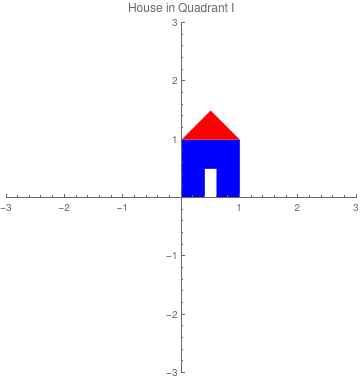
R . {1, 0}
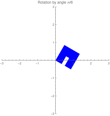
Now we rotate this unit square by 60°. We can use transposed matrix from the previous part as the rotation matrix. \begin{align*} \begin{bmatrix} X & Y \end{bmatrix} &= \begin{bmatrix} 0 & 0 \end{bmatrix} \,{\bf R}^{\mathrm T} = \begin{bmatrix} 0 & 0 \end{bmatrix} , \\ \begin{bmatrix} X & Y \end{bmatrix} &= \begin{bmatrix} 1 & 0 \end{bmatrix} \,{\bf R} = \begin{bmatrix} \frac{1}{2} & \frac{\sqrt{3}}{2} \end{bmatrix} \\ \begin{bmatrix} X & Y \end{bmatrix} &= \begin{bmatrix} 1 & 1 \end{bmatrix} \,{\bf R}^{\mathrm T} = \begin{bmatrix} \frac{1- \sqrt{3}}{2} & -\frac{1+\sqrt{3}}{2} \end{bmatrix} , \\ \begin{bmatrix} X & Y \end{bmatrix} &= \begin{bmatrix} 0 & 1 \end{bmatrix} \,{\bf R}^{\mathrm T} = \begin{bmatrix} -\frac{\sqrt{3}}{2} & \frac{1}{2}\end{bmatrix} . \end{align*}
In order to introduce polar coordinates, start with a point O in the plane ℝ² called the pole (we will always identify this point with the origin). From the pole, draw a ray, called the initial ray (we will always draw this ray horizontally, identifying it with the positive abscissa). A point P in the plane is determined by the distance r that P is from O, and the angle θ formed between the initial ray and the segment \( \displaystyle \quad \overline{OP} \quad \) (measured counter-clockwise). We record the distance and angle as an ordered pair (r, θ). This is illustrated in the following figure:

|
point = Graphics[{PointSize[0.02], Pink, Point[{1/2, Sqrt[3]/2}]}];
or = Graphics[{PointSize[0.02], Blue, Point[{0, 0}]}];
xar = Graphics[{Blue, Arrowheads[0.1], Arrow[{{0, 0}, {1, 0}}]}];
line = Graphics[{Black, Thick, Line[{{0, 0}, {1/2, Sqrt[3]/2}}]}];
txt = Graphics[{Black,
Text[Style["O", FontSize -> 18, Bold], {0, -0.5}],
Text[Style["r", FontSize -> 18, Bold], {0.2, 0.5}],
Text[Style["P = P(r, \[Theta])", FontSize -> 18, Bold], {0.5,
0.94}], Text[
Style["\[Theta]", FontSize -> 18, Bold], {0.56, 0.45}]}];
circle = Graphics[Circle[{0, 0}, 0.6, {0, Pi/3}]];
ar = Graphics[{Black, Arrowheads[0.04],
Arrow[{{0.32, 0.5059}, {0.3, 0.519}}]}];
Show[txt, xar, line, point, or, circle, ar]
|
Conversion between rectangular and polar coordinates are based of the relations: \[ \begin{split} x &= r\,\cos\theta , \\ y &= r\,\sin\theta , \qquad 0 \le r <\infty , \quad 0 \le \theta < 2\pi . \end{split} \] and \[ r = +\sqrt{x^2 + y^2} , \qquad \tan\theta = \frac{y}{x} . \]
We demonstrate advantages of polar coordinates with rotations figures. Although the classical equation of the heart/cardioid in polar coordinates is r = 1` - cosθ, we consider another equation of the same curve in Cartersian coordinates: \[ r = \frac{\sin t\,\sqrt{|\cos t |}}{\sin t + \frac{7}{5}} -2\,\sin t + 2 \qquad (0 \le t < 2\pi ). \tag{2.1} \]

|

|

|
PolarPlot[
Cos[t] Sqrt[Abs[Sin[t]]]/(Cos[t] + 7/5) - 2*Cos[t] + 2,
{t, 0, 2 Pi}, PlotStyle -> {Red, Thick}, Axes -> False
]
|

|
PolarPlot[-Cos[t] Sqrt[Abs[Sin[t]]]/(-Cos[t] + 7/5) + 2*Cos[t] +
2, {t, 0, 2 Pi}, PlotStyle -> {Purple, Thick}, Axes -> False]
|

|
PolarPlot[
Sin[t + Pi/3] Sqrt[Abs[Cos[t + Pi/3]]]/(Sin[t + Pi/3] + 7/5) -
2*Sin[t + Pi/3] + 2, {t, 0, 2 Pi}, PlotStyle -> {Blue, Thick},
Axes -> False]
|
Compositions
We now consider a case when one rotation is followed by another one. Suppose a rotation of the initial coordinate frame (points fixed) through an angle α is followed by a rotation of the resulting coordinate frame through an angle β. Clearly the result is a rotation of the initial coordinate frame (points fixed) through an angle α + β, as illustrated in Figure 4.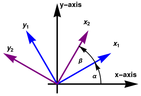
We consider a sequence of rotations when the initial coordinate frame (points fixed) through an angle α is followed by a rotation of the resulting coordinate frame through an angle β. Clearly the result is a rotation of the initial coordinate system (points fixed) through an angle of α + β, as illustratrated in Figure 4. The corresponding matrices of rotation are
Examples
|
\[ \frac{1}{2} \begin{bmatrix} \sqrt{3} & -1 \\ 1 & \sqrt{3} \end{bmatrix} \] |
|
|
|
\[ \frac{1}{2} \begin{bmatrix} -\sqrt{3} & -1 \\ 1 & -\sqrt{3} \end{bmatrix} \] |
|
|
|
\[ \frac{1}{2} \begin{bmatrix} 0 & -1 \\ 1 & \phantom{-}0 \end{bmatrix} \] |
|
|
|
\[ \frac{1}{2} \begin{bmatrix} \phantom{-}0 & 1 \\ -1 & 0 \end{bmatrix} \] |
|
Summary
| Type | angle θ | matrix | ||
|---|---|---|---|---|
| Rotation | 0° | \( \displaystyle \begin{bmatrix} 1&0 \\ 0&1 \end{bmatrix} \) | ||
| Rotation | 30° = π/6 | \( \displaystyle \frac{1}{2} \begin{bmatrix} \sqrt{3}&-1 \\ 1&\sqrt{3} \end{bmatrix} \) | ||
| Rotation | 45° = π/4 | \( \displaystyle \frac{\sqrt{2}}{2} \begin{bmatrix} 1&-1 \\ 1&1 \end{bmatrix} \) | ||
| Rotation | 60° = π/3 | \( \displaystyle \frac{1}{2} \begin{bmatrix} 1&-\sqrt{3} \\ \sqrt{3}&1 \end{bmatrix} \) | ||
| Rotation | 90° = π/2 | \( \displaystyle \begin{bmatrix} 0&1 \\ 1&0 \end{bmatrix} \) | ||
| Rotation | 120° = 2π/3 | \( \displaystyle \frac{1}{2} \begin{bmatrix} -1&-\sqrt{3} \\ \sqrt{3}&-1 \end{bmatrix} \) | ||
| Rotation | 135° = 3π/4 | \( \displaystyle \frac{\sqrt{2}}{2} \begin{bmatrix} -1&-1 \\ 1&-1 \end{bmatrix} \) | ||
| Rotation | 150° = 5π/6 | \( \displaystyle \frac{1}{2} \begin{bmatrix} -\sqrt{3}&-1 \\ 1&-\sqrt{3} \end{bmatrix} \) | ||
| Rotation | 180° = π | \( \displaystyle \begin{bmatrix} -1&0 \\ 0&-1 \end{bmatrix} \) |
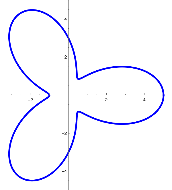
F = (2*Cos[3*t] + 3)*Cos[t];
G = (2*Cos[3*t] + 3)*Sin[t];
origPlot = ParametricPlot[{F, G}, {t, 0, 2*Pi}, PlotStyle -> {Blue, Thickness[0.01]}]
centerPlot = ListPlot[{Flatten[center]}, PlotMarkers -> {"+", Medium}];
sho2 = Show[rotPlot, centerPlot, PlotRange -> All]
|
|
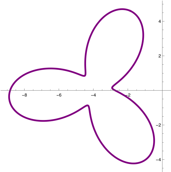
An alternative method
G = (2*Cos[3*t] + 3)*Sin[t];
origPlot = ParametricPlot[{F, G}, {t, 0, 2*Pi}, PlotStyle -> {Blue, Thickness[0.01]}];
P = {F, G}; center = {-2, -3}; Q = R . (P - center) + center; (* We don't need to flatten Q here *)
The latter figure clearly depicts the rotation of the parametric curve. Now let us animate the rotation so all intermediate curves will be visible.
G = (2*Cos[3*t] + 2)*1*Sin[t];
origPlot = ParametricPlot[{F, G}, {t, 0, 2*Pi}, PlotStyle -> {Blue, Thickness[0.01]}];
P = {{F}, {G}};
R = {{Cos[a], -Sin[a]}, {Sin[a], Cos[a]}};
center = {{-2}, {-3}};
QP = R.(P - center) + center;
centerPlot2 = Graphics[{Red, PointSize -> Medium, Point[{-2, -3}]}];
rotPlot = ParametricPlot[Flatten[Q], {t, 0, 2*Pi}, PlotStyle -> {Purple, Thickness[0.01]}]; anim2 = Animate[QPE = Evaluate[QP /. {a -> theta}]; QPEPlot = ParametricPlot[Flatten[QPE], {t, 0, 2*Pi}, PlotStyle -> {Black, Thickness[0.01]}]; Show[origPlot, QPEPlot, rotPlot, centerPlot2, PlotRange -> {{-10, 10}, {-10, 10}}], {{theta, 0, a}, 0, 2*Pi, Pi/16}, AnimationRepetitions -> Infinity ]
|
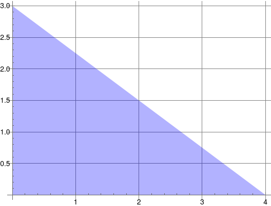
tri = Triangle[{{0, 0}, {4, 0}, {0, 3}}];
triRt = Graphics[Style[tri, Opacity[.3], Blue], Axes -> True,
GridLines -> Automatic]
|
|
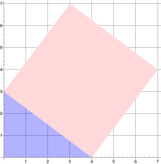
angle = ArcTan[-(3/4)];
redSq = Graphics[{LightRed,
Translate[
Rotate[Rectangle[{0, 0}, {5, 5}],
angle, {0, 0}], {4, 6} - {5 Cos[angle], -5 Sin[angle]}]}];
Show[triRt, redSq]
|
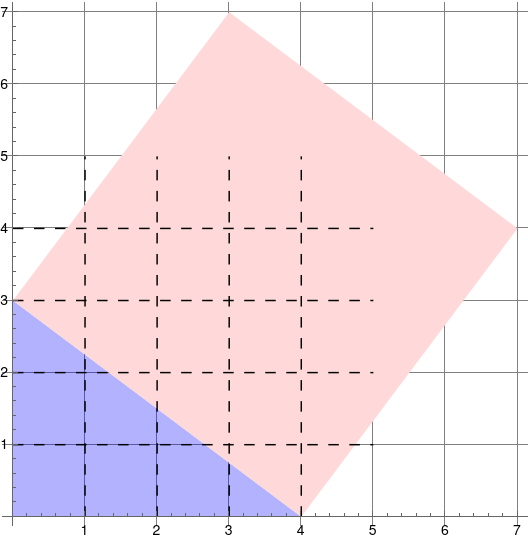
We need the grid to occupy the 5x5 red box. Below this is done in three steps. First we define the center of the grid
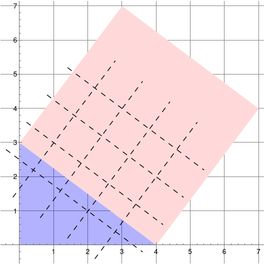
Now, using Translate, we move the grid northeast until it is inside the red square.
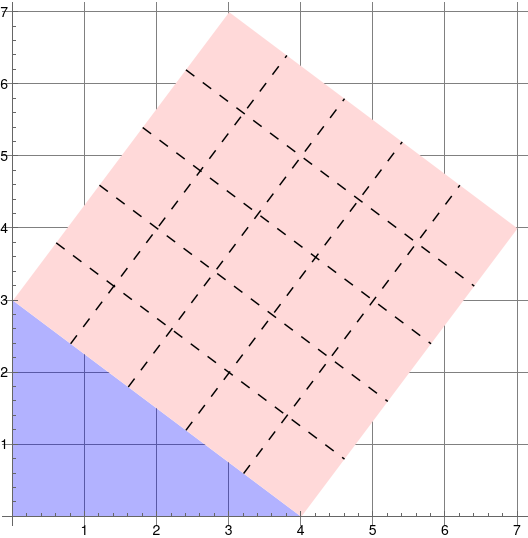
Note that using the coordinates indicated by the gridlines we can describe the beginning and ending positions of the square of dashed lines. It seems to me that there may be a matrix operation you might see that I do not which would simplify this. ■
Reflections
A rotation in the plane is closely related to reflection operation---a transformation that produces a mirror image of an object relative to anaxis of reflection (which is a fixed point for this transformation). Every rotation by angle θ can be formed by a pair of reflections. Suppose we have two lines (through the origin) L₁ and L₂ having angle θ between them. An arbitrary point P on the plane can be rotated by angle 2θ by reflecting P with respect to L₁ into P₁, which then is reflected into point P₂ with respect to line L₂.Let a reflection about a line L through the origin which makes an angle θ with the abscissa (x-axis) be denoted as Ref(θ). Suppose that these reflections operate on all points on the plane, and let these points be represented by position vectors. Then a reflection can be acomplished by applying orthogonal matrix (from left on column vectors or from right on row vectors) that performs mirrowing about the line that passes through the origin and is perpendicular to the unit vector \( \displaystyle \ \hat{\bf n} = \left( n_x, n_y \right) \ \) is given by
Using Eq.\eqref{EqReflection.1}, we derive
| Type | angle θ | matrix | ||
|---|---|---|---|---|
| Reflection | 0° | \( \displaystyle \begin{bmatrix} 1&0 \\ 0&-1 \end{bmatrix} \) | ||
| Reflection | 30° = π/6 | \( \displaystyle \frac{1}{2} \begin{bmatrix} 1&\sqrt{3} \\ 1\sqrt{3} & -1 \end{bmatrix} \) | ||
| Reflection | 45° = π/4 | \( \displaystyle \begin{bmatrix} 0&1 \\ 1&0 \end{bmatrix} \) | ||
| Reflection | 60° = π/3 | \( \displaystyle \frac{1}{2} \begin{bmatrix} -1&\sqrt{3} \\ \sqrt{3}&1 \end{bmatrix} \) | ||
| Reflection | 90° = π/2 | \( \displaystyle \begin{bmatrix} -1&0 \\ 0&1 \end{bmatrix} \) | ||
| Reflection | 120° = 2π/3 | \( \displaystyle \frac{1}{2} \begin{bmatrix} -1&\sqrt{3} \\ \sqrt{3} &1 \end{bmatrix} \) | ||
| Reflection | 135° = 3π/4 | \( \displaystyle \begin{bmatrix} 0&-1 \\ -1&0 \end{bmatrix} \) | ||
| Reflection | 150° = 5π/6 | \( \displaystyle \frac{1}{2} \begin{bmatrix} 1&-\sqrt{3} \\ \sqrt{3}&-1 \end{bmatrix} \) | ||
| Reflection | 180° = π | \( \displaystyle \begin{bmatrix} 1&0 \\ 0&1 \end{bmatrix} \) |
- Consider the point P(2,1). Without using matrix multiplication, find the resulting point undr rotation about the origin by angles π/2 and π/4.
- Given a point P on the plane ℝ², let Q be the point corresponding to the rotation of P in counterclockwise direction about the origin through an angle θ. Let R be the point corresponding to the rotation of Q in counterclockwise direction about the origin through an angle ϕ. Verify that \[ \mathbf{R}[\phi ]\,\mathbf{R}[\theta ] = \mathbf{R}[\phi + \theta ] , \] where R[θ] is the rotation matrix according to formula (1). Does it mean that products of rotation matrices are commutative?
- Find the coordinates of the point Q corresponding to the point P(3, 2) that has been rotated in counterclockwise direction about the origin through an angle θ = 2π/3.
- Anton, Howard (2005), Elementary Linear Algebra (Applications Version) (9th ed.), Wiley International
- Dunn, F. and Parberry, I. (2002). 3D math primer for graphics and game development. Plano, Tex.: Wordware Pub.
- Coolidge, J.L., The Origin of Polar Coordinates, American Mathematical Monthly. Mathematical Association of America: 1952, volume 59, issue 2, pp. 78–85. doi:10.2307/2307104.
- Foley, James D.; van Dam, Andries; Feiner, Steven K.; Hughes, John F. (1991), Computer Graphics: Principles and Practice (2nd ed.), Reading: Addison-Wesley, ISBN 0-201-12110-7
- Matrices and Linear Transformations
- Pen and Paper Science
- Rogers, D.F., Adams, J. A., Mathematical Elements for Computer Graphics, McGraw-Hill Science/Engineering/Math, 1989.