This section is divided into a number of subsections, links to which are:

Although physical phase space can extend to thousands of dimensions, our minds are incapable of thinking even in five dimensions—we have no ability to visualize such things. It is impossible to do physics in high dimensions without having the right tools and symbols with which to work. Cross product is an important tool applied only in three dimensional vector space. In Euclidean space, a cross product is related to areas of parallelograms and volumes of parallelepipeds. Thus, it opens the door of high dimensional math and physics, including tensors and wedge products.

In 1881, Josiah Willard Gibbs (1839--1903), and independently Oliver Heaviside (1850--1925), introduced the notation for both the dot product and the cross product using a period (a • b) and an "×" (a × b), respectively, to denote them.

In 1877, to emphasize the fact that the result of a dot product is a scalar while the result of a cross product is a vector, William Kingdon Clifford (1845--1879) coined the alternative names scalar product and vector product for the two operations. These alternative names are still widely used in the literature.

Vector or Cross product

It is well-known that a vector space can be equipped with a product operation (besides vector addition) only for dimensions 1 and 2. The cross product is a successful attempt to implement the product in a three-dimensional vector space, but without the commutative property of multiplication. On the other hand, the outer product assigns a matrix to two vectors of arbitrary size.

For any two vectors in ℝ³,

$\displaystyle {\bf a} = \left[ a_1 , a_2 , a_3 \right]$ and

$\displaystyle {\bf b} = \left[ b_1 , b_2 , b_3 \right] ,$ their cross product is the vector (written in a column form for convenience)

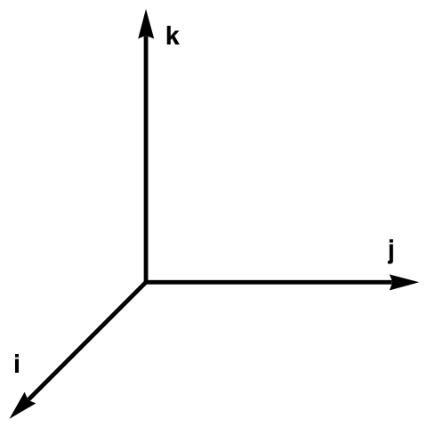
$\begin{equation} \label{EqCross.1} {\bf a} \times {\bf b} = \det \begin{bmatrix} \hat{\bf e}_1 & \hat{\bf e}_2 & \hat{\bf e}_3 \\ a_1 & a_2 & a_3 \\ b_1 & b_2 & b_3 \end{bmatrix} = \begin{bmatrix} a_2 b_3 - a_3 b_2 \\ a_3 b_1 - a_1 b_3 \\ a_1 b_2 - a_2 b_1 \end{bmatrix} . \end{equation}$

Here

$\displaystyle \hat{\bf e}_1 , \ \hat{\bf e}_2 , \ \hat{\bf e}_3 \$ are unit vectors in ℝ³ that are also usually denoted by i, j, and k, respectively.

Clear[e, e1, e2, e3]; e = {e1, e2, e3}; a = {a1, a2, a3}; b = {b1, b2, b3}; MatrixForm[{e, a, b}]; Det[{e, a, b}]

a3 b2 e1 + a2 b3 e1 + a3 b1 e2 - a1 b3 e2 - a2 b1 e3 + a1 b2 e3

Coefficient[Det[{e, a, b}], #] & /@ {e1, e2, e3}

{-a3 b2 + a2 b3, a3 b1 - a1 b3, -a2 b1 + a1 b2}

Cross[a, b]

{-{-a3 b2 + a2 b3, a3 b1 - a1 b3, -a2 b1 + a1 b2}a3 b2 + a2 b3, a3 b1 - a1 b3, -a2 b1 + a1 b2}

TrueQ[% == %%]

True

Cross-product of two vectors together with these vectors form so called right-handed system.

Three vectors, u, v, w, form a right-handed system if when you extend the thumb of your right hand in the direction of u and your index finger in the direction of v, your relaxed middle finger points roughly in the direction of w.

The special basis vectors i = (1, 0, 0), j = (0, 1, 0), and k = (0, 0, 1) form a right-handed system in ℝ³. Thus, if the thumb of your right hand points along the x-axis and your index finger points along the y-axis, your middle finger should point along the z-axis. When all three vectors lie in a plane, then we say that the vectors are coplanar. In this case, the system is neither right-handed nor left-handed.

ii1 = Graphics[{Arrowheads[0.07], Thickness[0.01], Arrow[{{0, 0}, {-0.5, -0.5}}]}]; jj1 = Graphics[{Arrowheads[0.07], Thickness[0.01], Arrow[{{0, 0}, {1, 0}}]}]; kk1 = Graphics[{Arrowheads[0.07], Thickness[0.01], Arrow[{{0, 0}, {0, 1}}]}]; ti1 = Graphics[ Text[Style["i", Bold, FontSize -> 12], {-0.47, -0.3}]]; tj1 = Graphics[Text[Style["j", Bold, FontSize -> 12], {0.9, 0.12}]]; tk1 = Graphics[ Text[Style["k", Bold, FontSize -> 12], {0.1, 0.9}]]; rhs = Labeled[Show[ii1, jj1, kk1, ti1, tj1, tk1, AspectRatio -> 1], "Figure 1:\nRight-handed system(air force]"];

ii2 = Graphics[{Arrowheads[0.07], Thickness[0.01], Arrow[{{0, 0}, {1.0, 0}}]}]; jj2 = Graphics[{Arrowheads[0.07], Thickness[0.01], Arrow[{{0, 0}, {-0.5, 0.5}}]}]; kk2 = Graphics[{Arrowheads[0.07], Thickness[0.01], Arrow[{{0, 0}, {0, -1}}]}]; ti2 = Graphics[Text[Style["x", Bold, FontSize -> 12], {0.9, 0.1}]]; tj2 = Graphics[ Text[Style["y", Bold, FontSize -> 12], {-0.35, 0.45}]]; tk2 = Graphics[Text[Style["z", Bold, FontSize -> 12], {0.1, -0.9}]]; lhs = Labeled[Show[ii2, jj2, kk2, ti2, tj2, tk2, AspectRatio -> 1], "Figure 2:\nLeft-handed system(navy)"];
Grid[{{rhs, Spacer[140], lhs}}]

Figure 1: Right-handed system (air force).

Besides algebraic definition of the cross product, it is possible to give a geometrical one.

Theorem 1: Let a and b be two vectors in ℝ³. Their cross product, written a × b, is the vector defined by the following three rules.

The length of cross product can be defined as
$\begin{equation} \label{EqCross.2} {\bf a} \times {\bf b} = \| {\bf a} \| \, \| {\bf b} \|\,\sin (\theta )\,{\bf n} , \end{equation}$
where
- θ is the angle between a and b in the plane containing them (hence, it is between 0 and π);
- ∥ x ∥ is the Euclidean norm, so $\displaystyle \| {\bf x} \| = \| (x_1 , x_2 , x_3 )\| = \sqrt{x_1^2 + x_2^2 + x_3^2} ;$
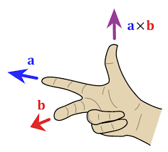
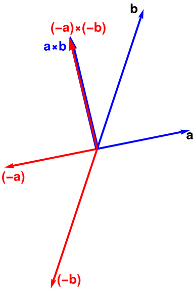
- n is a unit vector perpendicular to the plane containing a and b, with direction such that the ordered set (a, b, n) is positively-oriented. Conventionally, direction of n is given by the right-hand rule, where one simply points the forefinger of the right hand in the direction of a and the middle finger in the direction of b. Then, the vector n is coming out of the thumb (see the adjacent picture).
It is orthogonal to both a and b.
The vectors a, b, and a × b, in that order, form a right-handed system.

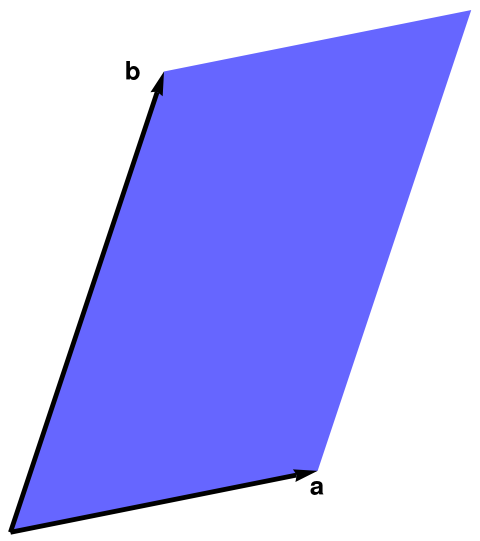
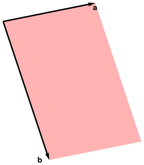
We note that the length of the cross product, ∥ a × b ∥ = ∥ a ∥ ∥ b ∥ sin(θ) , given by the formula

$\eqref{EqCross.2}$ , is the area of the parallelogram determined by a and b.

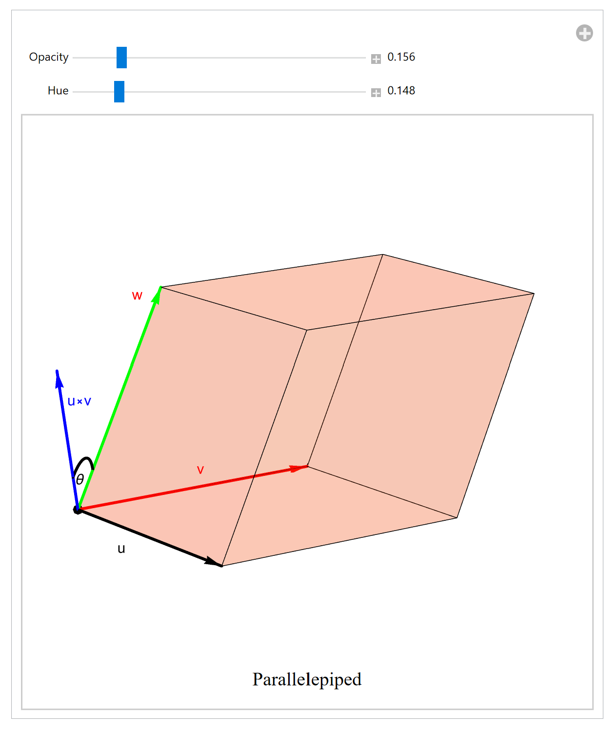
We plot with Mathematica cross product of two vectors using DynamicModule command so you can see the value of cross product, which is the area of parallelogram (in blue for the acute angle, pink for the obtuse angle) formed by two given vectors. You can manipulate the plot in Mathematica by dragging the arrowheads.

mani1 = Manipulate[ DynamicModule[{vv, ww, angles, cros}, vv = Normalize[v]; ww = Normalize[w]; cros = First[PadLeft[v, 3]\[Cross]PadLeft[w, 3]]; angles = Sort[N@{ArcTan @@ vv, ArcTan @@ ww}]; Graphics[{{If[ showPar, {If[cros > 0, LightBlue, LightRed], Polygon[{{0, 0}, v, v + w, w}]}]}, {If[cros < 0, Blue, Red], Circle[{0, 0}, .3, If[-Subtract @@ angles < \[Pi], angles, Reverse[angles] + {0, 2 \[Pi]}]]}, {GrayLevel[0], Arrow[{{0, 0}, v}]}, {GrayLevel[0], Arrow[{{0, 0}, w}]}, {If[cros > 0, RGBColor[1, 0.47, 0], RGBColor[0.4156862745098039, 0.3529411764705882, 0.803921568627451]], Arrow[{{0, 0}, cros {-1/2, -1/2}}]}, Text["\!$\*OverscriptBox[\(v$, $\[RightVector]$]\)", v .65, {.3, 1}], Text["\!$\*OverscriptBox[\(w$, $\[RightVector]$]\)", 3 w/4, {1.75, 1}], Text["\!$\*OverscriptBox[\(v$, $\[RightVector]$]\)\[Cross]\!\ $\*OverscriptBox[\(w$, $\[RightVector]$]\)", If[cros < 0, cros {-.65, -.65}, cros {-1/2, -1/2}], {1, 1}]}, Axes -> True, Ticks -> True, PlotRange -> 3, ImageSize -> {400, 400}, PlotLabel -> Grid[{{If[cros > 0, Style["acute or obtuse angle", RGBColor[1, 0.47, 0]], Style["reflex angle", RGBColor[0.4156862745098039, 0.3529411764705882, 0.803921568627451]]], Norm["\!$\*OverscriptBox[\(v$, \ $\[RightVector]$]\)\[Cross]\!$\*OverscriptBox[\(w$, $\ \[RightVector]$]\)"] == DecimalForm[ Abs[cros], {4, 3}]}, {"\!$\*OverscriptBox[\(v$, $\[RightVector]$]\)", v}, {"\!$\*OverscriptBox[\(w$, $\[RightVector]$]\)", w}}, ItemSize -> 10]]], {{showPar, True, "show parallelogram"}, {True, False}}, {{v,(*{1.255881,0.83}*){1., 0.5}}, {-3, -3}, {3, 3}, Locator, Appearance -> None, Exclusions -> {0, 0}}, {{w,(*{0.459599, 1.1}*){0.27, 1.135}}, {-3, -3}, {3, 3}, Locator, Appearance -> None, Exclusions -> {0, 0}}]

par = Graphics[{Lighter[Pink, 0.4], Parallelogram[{0, 0}, {{1, 0.2}, {0.5, -1.5}}]}];
ar1 = Graphics[{Black, Arrowheads[0.05], Thickness[0.01], Arrow[{{0, 0}, {1, 0.2}}]}];
ar2 = Graphics[{Black, Arrowheads[0.05], Thickness[0.01], Arrow[{{0, 0}, {0.5, -1.5}}]}];
txt1 = Graphics[{Black, Text[Style["a", 20, Bold], {1, 0.15}]}]; txt2 = Graphics[{Black, Text[Style["b", 20, Bold], {0.4, -1.5}]}]; Show[par, ar1, ar2, txt1, txt2]

par = Graphics[{Lighter[Blue, 0.4], Parallelogram[{0, 0}, {{1, 0.2}, {0.5, 1.5}}]}];
ar1 = Graphics[{Black, Arrowheads[0.05], Thickness[0.01], Arrow[{{0, 0}, {1, 0.2}}]}];
ar2 = Graphics[{Black, Arrowheads[0.05], Thickness[0.01], Arrow[{{0, 0}, {0.5, 1.5}}]}];
txt1 = Graphics[{Black, Text[Style["a", 20, Bold], {1, 0.15}]}]; txt2 = Graphics[{Black, Text[Style["b", 20, Bold], {0.4, 1.5}]}]; Show[par, ar1, ar2, txt1, txt2]

Figure 5: Area of parallelogram in blue.

Figure 6: Area of parallelogram in pink.

Example 1: Let us consider two vectors (that we write as column vectors):

${\bf a} = \begin{pmatrix} 1 \\ 2 \\ 0 \end{pmatrix} \qquad \mbox{and} \qquad {\bf b} = \begin{pmatrix} -1 \\ \phantom{-}1 \\ \phantom{-}1 \end{pmatrix}$ Although we can use Eq.(1) to determine components of their cross product, we dedicate this job to Mathematica:

a = {1, 2, 0} ; b = {-1, 1, 1};
c = Cross[a, b]

{2, -1, 3}

Or, equivalently, Mathematica has an operator for Cross

a\[Cross]b

{2, -1, 3}

${\bf c} = {\bf a} \times {\bf b} = \begin{pmatrix} 1 \\ 2 \\ 0 \end{pmatrix} \times \begin{pmatrix} -1 \\ \phantom{-}1 \\ \phantom{-}1 \end{pmatrix} = \begin{pmatrix} \phantom{-}2 \\ -1 \\ \phantom{-}3 \end{pmatrix} .$ The length of cross product of two vectors is equal to the area of the parallelogram spanned on these vectors; therefore, we have

$| {\bf c} | = | {\bf a} \times {\bf b} | = \sqrt{2^2 + (-1)^2 + 3^2} = \sqrt{14} .$

Norm[%]

Sqrt[14]

N[Norm[c]]

3.74166

Norm[a]

Sqrt[5]

Norm[b]

Sqrt[3]

para = Graphics[{Lighter[Purple, 0.1], Parallelogram[{0, 0}, {{1, 0.2}, {-0.5, 1.5}}]}];
Labeled[Graphics[para, Axes -> True, Ticks -> True, Epilog -> Text["Area of parallelogram:\n= Determinant{v,w}\n= Length of the cross product{v,w}\n= 1", {.65, .85}]], "Area of Parallelogram"]

Area[para]

{Norm[a], Norm[b]}

{Sqrt[5], Sqrt[3]}

Since norms of these two vectors are

$\| {\bf a} \| = \sqrt{5} \qquad \mbox{and} \qquad \| {\bf b} \| = \sqrt{3} ,$

Det[{{1., 0.5}, {0.27, 1.135}}]

we find angle between these two vectors:

$\theta = \mbox{arccos} \left( \frac{\sqrt{14}}{\sqrt{15}} \right) \approx \mbox{arccos} \left( 0.966092 \right) \approx 0.261157 .$

ArcCos[Sqrt[14]/Sqrt[15]] // N

0.261157

N[Sqrt[14/15]]

0.966092

N[ArcCos[Sqrt[14/15]]]

0.261157

End of Example 1

■

Despite that the cross product is identified uniquely by two entries, there is something very peculiar about the vector u × v. If u and v are orthogonal unit vectors, then the vectors u, v, u × v form a right-handed coordinate system. But if R ∈ ℝ^3×3 is the linear transformation (whch is 3×3 matrix with real entries) that mirrors vectors in the u, v plane, then { R u, R v, R u×v } = { u, v, −u×v } forms a left-handed coordinate system. In general, the cross product obeys the following identity under matrix transformation:

$\begin{equation} \label{EqCross.3} \left( {\bf M}\,{\bf u} \right) \times \left( {\bf M}\,{\bf v} \right) = (\det {\bf M} )\,{\bf M}^{-\mathrm{T}} \left( {\bf u} \times {\bf v} \right) , \end{equation}$

where M is a 3×3 matrix and M^−T is the transpose of the inverse matrix.

Thus, cross product u×v is not really transformed as a vector. This anomaly should alert us to the fact that cross product is not really a true vector. In fact, cross product is transformed more like a tensor than a vector.

ar1 = Graphics[{Blue, Arrowheads[0.05], Thickness[0.01], Arrow[{{0, 0}, {1, 0.2}}]}];
ar2 = Graphics[{Blue, Arrowheads[0.05], Thickness[0.01], Arrow[{{0, 0}, {0.5, 1.5}}]}];
ar1m = Graphics[{Red, Arrowheads[0.05], Thickness[0.01], Arrow[{{0, 0}, {-1, -0.2}}]}];
ar2m = Graphics[{Red, Arrowheads[0.05], Thickness[0.01], Arrow[{{0, 0}, {-0.5, -1.5}}]}];
ar = Graphics[{Blue, Arrowheads[0.07], Thickness[0.02], Arrow[{{0, 0}, {-0.3, 1.2}}]}]; arr = Graphics[{Red, Arrowheads[0.07], Thickness[0.02], Arrow[{{0, 0}, {-0.3, 1.2}}]}];
txt1 = Graphics[{Black, Text[Style["a", 20, Bold], {1, 0.15}]}]; txt2 = Graphics[{Black, Text[Style["b", 20, Bold], {0.4, 1.5}]}]; txt1m = Graphics[{Red, Text[Style["(-a)", 20, Bold], {-0.9, -0.3}]}]; txt2m = Graphics[{Red, Text[Style["(-b)", 20, Bold], {-0.3, -1.4}]}];
tm = Graphics[{Red, Text[Style["(-a)\[Cross](-b)", 20, Bold], {-0.2, 1.3}]}]; t = Graphics[{Blue, Text[Style["a\[Cross]b", 20, Bold], {-0.45, 1.1}]}];
Show[ar1, ar2, ar1m, ar2m, txt1, txt2, txt1m, txt2m, ar, arr, t, tm]

Note when BOTH vectors change sign, the cross product is unchanged. However, this is not true when only one vector changes sign in cross product.

Example 2: Let us consider two vectors a = [ 2, −1, −1 ] and b = [ −1, 2, 1 ]. Their cross product is

${\bf a} \times {\bf b} = \begin{pmatrix} \phantom{-}2 \\ -1 \\ -1 \end{pmatrix} \times \begin{pmatrix} -1 \\ \phantom{-}2 \\ \phantom{-}1 \end{pmatrix} = \begin{pmatrix} \phantom{-}1 \\ -1 \\ \phantom{-}3 \end{pmatrix} .$

ab =Cross[{2, -1, -1}, {-1, 2, 1}]

{1, -1, 3}

Let us consider the following transformation:

${\bf M} = \begin{bmatrix} 3 & -1 & 11 \\ 2 & \phantom{-}2 & -3 \\ 2 & \phantom{-}1 & \phantom{-}1 \end{bmatrix} .$

M = {{3, -1, 11}, {2, 2, -3}, {2, 1, 1}}; Det[M]

Since det(M) = 1, its transposed inverse is

${\bf M}^{-{\mathrm T}} = \begin{bmatrix} \phantom{-}5 & -8 & -2 \\ 12 & -19 & -5 \\ -19 & \phantom{-}31 & \phantom{-}8 \end{bmatrix} .$

sM = Transpose[Inverse[M]]

{{5, -8, -2}, {12, -19, -5}, {-19, 31, 8}}

MatrixForm[sM]

$\displaystyle \begin{pmatrix} 5 & -8 & -2 \\ 12 & -19 & -5 \\ -19 & 31 & 8 \end{pmatrix}$

Now we multiply given vectors a and b by matrix M:

${\bf M}\,{\bf a} = \begin{bmatrix} -4 \\ \phantom{-}5 \\ \phantom{-}2 \end{bmatrix} , \qquad {\bf M}\,{\bf b} = \begin{bmatrix} \phantom{-}6 \\ -1 \\ \phantom{-}1 \end{bmatrix} .$

M = {{3, -1, 11}, {2, 2, -3}, {2, 1, 1}} ;
a = {2, -1, -1} ;
Ma = M.a

{-4, 5, 2}

and

M = {{3, -1, 11}, {2, 2, -3}, {2, 1, 1}} ;
b = {-1, 2, 1};
Mb = M.b

{6, -1, 1}

Their cross product becomes

$\left( {\bf M}\,{\bf a} \right) \times \left( {\bf M}\,{\bf b} \right) = \begin{pmatrix} -4 \\ \phantom{-}5 \\ \phantom{-}2 \end{pmatrix} \times \begin{pmatrix} \phantom{-}6 \\ -1 \\ \phantom{-}1 \end{pmatrix} = \begin{pmatrix} \phantom{-}7 \\ \phantom{-}16 \\ -26 \end{pmatrix} .$

MMab = Cross[Ma, Mb]

{7, 16, -26}

On the other hand,

${\bf M}^{-\mathrm{T}} \left( {\bf a} \times {\bf b} \right) = \begin{pmatrix} \phantom{-}7 \\ \phantom{-}16 \\ -26 \end{pmatrix} .$

ab = {1, -1, 3};
sM = Transpose[Inverse[M]] ;
sM.ab

{7, 16, -26}

End of Example 2

■

We are interested in more general formula than Eq.(3). Suppose that a linear transformation is defined by a 3×3 matrix

${\bf P} = \begin{bmatrix} p_{1,1} & p_{1,2} & p_{1,3} \\ p_{2,1} & p_{2,2} & p_{2,3} \\ p_{3,1} & p_{3,2} & p_{3,3} \end{bmatrix} = \begin{bmatrix} {\bf p}_1 \\ {\bf p}_2 \\ {\bf p}_3 \end{bmatrix} ,$

where p₁, p₂, and p₃ are row vectors in matrix P. This matrix (as any 3×3 matrix) defines a linear transformation in ℝ^3×1 by multiplication from the left. Then a natural question arises whether it is possible to express a transformed cross product

$\left( {\bf P}\,{\bf v} \right) \times {\bf u}$

in terms of transformed cross product v × u, similar to Eq.(3). For example, if P is a diagonal matrix, then

$\left( \begin{bmatrix} \lambda_1 & 0 & 0 \\ 0 & \lambda_2 & 0 \\ 0&0& \lambda_3 \end{bmatrix} \,\begin{bmatrix} v_1 \\ v_2 \\ v_3 \end{bmatrix} \right) \times \begin{bmatrix} u_1 \\ u_2 \\ u_3 \end{bmatrix} = \begin{bmatrix} \lambda_2 v_2 u_3 - \lambda_3 v_3 u_2 \\ \lambda_1 v_1 u_3 - \lambda_3 v_3 u_1 \\ \lambda_1 v_1 u_2 - \lambda_2 v_2 u_1 \end{bmatrix} .$

This expression for diagonal matrix tells us that there is no simple formula for vector product (Pv) × u in terms of v × u because vector product is a bilinear transformation ℝ³ × ℝ³ ↦ ℝ³. On the other hand, if we fix vector u, then cross product becomes a linear transformation

$T({\bf v}) = {\bf v} \times {\bf u} = {\bf A}\,{\bf v} \qquad \Longrightarrow \qquad T\,:\ \mathbb{R}^3 \mapsto \mathbb{R}^3 .$

A square matrix A = [T] of this linear transformation depends on vector u:

${\bf A} = \begin{bmatrix} 0 & u_3 & -u_2 \\ - u_3 & 0 & u_1 \\ u_2 & -u_1 & 0\end{bmatrix} .$

This singular skew-symmetric matrix has one real eigenvalue λ₁ = 0 and two pure imaginary eigenvalues (j² = −1)

$\lambda_1 = 0, \qquad \lambda_{2,3} = \pm {\bf j} \sqrt{u_1^2 + u_2^2 + u_3^2} = \pm {\bf j}\,\| {\bf u} \| . .$

A = {{0, u3, -u2}, {-u3, 0, u1}, {u2, -u1, 0}};
Eigenvalues[A]

{0, -Sqrt[-u1^2 - u2^2 - u3^2], Sqrt[-u1^2 - u2^2 - u3^2]}

The null space of T is the line through the origin spanned by vector u and its image is the plane through the origin orthogonal to u.

One of the main motivations to use cross product comes from classical mechanics: A torque τ about a point due to a force F acting at another point at distance r is expressed through cross product: τ = r × F.

The cross product is convenient to define with the Levi-Civita symbol that was invented in the late 1800's by the Italian mathematician Tullio Levi-Civita (1873--1941), a student of Gregorio Ricci:

$\begin{equation} \label{EqCross.4} \varepsilon_{i,j,k} = \begin{cases} \phantom{-}0 , & \quad\mbox{if any two labels are the same}, \\ -1, & \quad \mbox{if }i,\, j,\,k \mbox{ is an odd permutation of 1, 2, 3}, \\ \phantom{-}1 , & \quad \mbox{if } i,\, j,\,k \mbox{ is an even permutation of 1, 2, 3}. \end{cases} \end{equation}$

The Levi-Civita symbol ε_ijk is a tensor of rank three and is anti-symmetric on each pair of indexes. The determinant of a matrix A with elements 𝑎_ij can be written in term of ε_ijk

$\det\begin{bmatrix} a_{11} & a_{12} & a_{13} \\ a_{21} & a_{22} & a_{23} \\ a_{31} & a_{32} & a_{33} \end{bmatrix} = \sum_{i,j=1}^3 \varepsilon_{ijk} a_{1i} a_{2j} a_{3k} = \varepsilon_{ijk} a_{1i} a_{2j} a_{3k} ,$

upon dropping sign of summation using the Einstein summation rule. The Levi-Civita symbol possesses the following properties

The Levi-Civita tensor has 3×3×3 = 27 components;
3 × (6+1) = 21 components are equal to 0;
3 components are equal to 1 = ε₁₂₃ = ε₂₃₁ = ε₃₂₁;
3 components are equal to −1 = ε₃₂₁ = ε₂₁₃ = ε₁₃₂.

Cross product in index notation using Levi-Civita symbol is

$\begin{equation} \label{EqCross.5} {\bf a} \times {\bf b} = \varepsilon_{ijk} \hat{\bf e}_i a_j b_k . \end{equation}$

Given two space vectors, a and b, we can find a third space vector c, called the cross product of a and b, and denoted by c = a × b. The magnitude of c is defined by |c| = |a| |b| sin(θ), where θ is the angle between a and b.

The direction of c is given by the right-hand rule: If a is turned to b (note the order in which a and b appear here) through the angle between a and b, a (right-handed) screw that is perpendicular to a and b will advance in the direction of a × b. This definition implies that

${\bf a} \times {\bf b} = - {\bf b} \times {\bf a} .$

This property is described by saying that the cross product is antisymmetric. The definition also implies that

${\bf a} \bullet \left( {\bf a} \times {\bf b}\right) = {\bf b} \bullet \left( {\bf a} \times {\bf b}\right) = {\bf 0} ,$

where • denotes dot product. That is, a × b is perpendicular to both a and b. The vector product has the following properties:

$\begin{align*} {\bf a} \times \left( \alpha {\bf b}\right) &= \left( \alpha {\bf a} \right) \times {\bf b} = \alpha \left( {\bf a} \times {\bf b}\right) , \\ {\bf a} \times \left( {\bf b} + {\bf c} \right) &= {\bf a} \times {\bf b} + {\bf a} \times {\bf c} , \\ {\bf a} \times {\bf a} &= {\bf 0} . \end{align*}$

Using these properties, we can write the vector product of two vectors in terms of their components. We are interested in a more general result valid in other coordinate systems as well. So, rather than using x, y, and z as subscripts for unit vectors, we use the numbers 1, 2, and 3. In that case, our results can also be used for spherical and cylindrical coordinates which we shall discuss shortly.

$\begin{align*} {\bf a} \times {\bf b} &= \left( \alpha_1 \hat{\bf e}_1 + \alpha_2 \hat{\bf e}_2 + \alpha_3 \hat{\bf e}_3 \right) \times \left( \beta_1 \hat{\bf e}_1 + \beta_2 \hat{\bf e}_2 + \beta_3 \hat{\bf e}_3 \right) \\ &= \alpha_1 \beta_1 \hat{\bf e}_1 \times \hat{\bf e}_1 + \alpha_1 \beta_2 \hat{\bf e}_1 \times \hat{\bf e}_2 + \alpha_1 \beta_3 \hat{\bf e}_1 \times \hat{\bf e}_3 \\ & \quad + \alpha_2 \beta_1 \hat{\bf e}_2 \times \hat{\bf e}_1 + \alpha_2 \beta_2 \hat{\bf e}_2 \times \hat{\bf e}_2 + \alpha_2 \beta_3 \hat{\bf e}_2 \times \hat{\bf e}_3 \\ & \quad + \alpha_3 \beta_1 \hat{\bf e}_3 \times \hat{\bf e}_1 + \alpha_3 \beta_2 \hat{\bf e}_3 \times \hat{\bf e}_2 + \alpha_3 \beta_3 \hat{\bf e}_3 \times \hat{\bf e}_3 \end{align*}$

Using the antisymmetry property of cross product, we have

$\hat{\bf e}_1 \times \hat{\bf e}_1 = \hat{\bf e}_2 \times \hat{\bf e}_2 = \hat{\bf e}_3 \times \hat{\bf e}_3 = {\bf 0}.$

Also, if we assume that

$\hat{\bf e}_1 , \ \hat{\bf e}_2 , \ \hat{\bf e}_3$ form a so-called right-handed set, i.e., if

$\begin{align} \notag \hat{\bf e}_1 \times \hat{\bf e}_2 &= - \hat{\bf e}_2 \times \hat{\bf e}_1 = \hat{\bf e}_3 , \\ \hat{\bf e}_1 \times \hat{\bf e}_3 &= - \hat{\bf e}_3 \times \hat{\bf e}_1 = - \hat{\bf e}_2 , \label{EqCross.6} \\ \hat{\bf e}_2 \times \hat{\bf e}_3 &= - \hat{\bf e}_3 \times \hat{\bf e}_2 = \hat{\bf e}_1 , \notag \end{align}$

then we obtain

${\bf a} \times {\bf b} = \left( \alpha_2 \beta_3 - \alpha_3 \beta_2 \right) \hat{\bf e}_1 + \left( \alpha_3 \beta_1 - \alpha_1 \beta_3 \right) \hat{\bf e}_2 + \left( \alpha_1 \beta_2 - \alpha_2 \beta_1 \right) \hat{\bf e}_3 .$

Theorem 3:

${\bf a} \times \left( {\bf b} \times {\bf c} \right) = {\bf b} \left( {\bf a}\bullet {\bf c} \right) - {\bf c} \left( {\bf a}\bullet {\bf b} \right) .$

Let

${\bf d} = {\bf a} \times \left( {\bf b} \times {\bf c} \right) ,$

then its m-th component is

$\begin{align*} d_m &= \varepsilon_{mni} a_n \left( \varepsilon_{ijk} b_j c_k \right) \\ &= \varepsilon_{mni} \varepsilon_{ijk} a_n b_j c_k = \left( \delta_{mj} \delta_{nk} - \delta_{mk} \delta_{nj} \right) a_n b_j c_k \\ &= b_m a_k c_k - c_m a_j b_j \\ &= \left[{\bf b} \left( {\bf a}\bullet {\bf c} \right) \right]_m - \left[ {\bf c} \left( {\bf a}\bullet {\bf b} \right) \right]_m . \end{align*}$

Example 3: We use Mathematica to prove the following properties of cross product. Although Matheatica is a computer algebra system, so it allows to use algebraic expressions for manipulations, we illustrate its capability on numerical example. Therefore, we utilize the rows of the following vectors, a, b, and c used in the previous Example:

${\bf a} = \begin{pmatrix} \phantom{-}2 \\ -1 \\ -1 \end{pmatrix} , \qquad {\bf b} = \begin{pmatrix} -1 \\ \phantom{-}2 \\ \phantom{-}1 \end{pmatrix} , \qquad {\bf c} = {\bf a} \times {\bf b} = \begin{pmatrix} \phantom{-}1 \\ -1 \\ \phantom{-}3 \end{pmatrix} ,$

a = {2, -1, -1};
b = {-1, 2, 1};
c = Cross[a, b];

a × a = 0.
a × b = −b × a.
(ka) × b = k(a × b) = a × (kb) for any real scalar k ∈ ℝ.
a × (b + c) = a × b + a × c.
a • (b × c) = b • (c × a) = c • (a × b).
a × (b × c) + b × (c × a) + c × (a × b) = 0.
a × (b × c) = b(c • a) − c(a • b).
(a × b) × c = b(c • a) − a(b • c).

Solution.

a × a = 0.
a\[Cross]a

{0, 0, 0}
a × b = −b × a.
TrueQ[a\[Cross]b == -b\[Cross]a]

True
(ka) × b = k(a × b) = a × (kb) for any real scalar k ∈ ℝ.
TrueQ[(k a)\[Cross]b == k (a\[Cross]b) == a\[Cross] (k b)]

True
a × (b + c) = a × b + a × c.
TrueQ[a*(b + c) == a*b + a*c]

True
a • (b × c) = b • (c × a) = c • (a × b).
TrueQ[a . (b*c) == b . (c*a) == c . (a*b)]

True
a × (b × c) + b × (c × a) + c × (a × b) = 0.
TrueQ[a\[Cross](b\[Cross]c) + b\[Cross](c\[Cross]a) + c\[Cross](a\[Cross]b) == {0, 0, 0}]

True
a × (b × c) = b(c • a) − c(a • b).
TrueQ[a\[Cross](b\[Cross]c) == b (c . a) \[Minus] c (a . b)]

True
(a × b) × c = b(c • a) − a(b • c).
TrueQ[(a\[Cross]b)\[Cross]c == b (c . a) \[Minus] a (b . c)]

True

End of Example 3

■

The property of cross product, a × (b × c) = b(c • a) − c(a • b), discussed in the previous example, can be used to prove the identity involving the gradient operator ∇:

$\begin{align*} \nabla \times \left( \nabla \times {\bf f} \right) &= \nabla \left( \nabla \bullet {\bf f} \right) - \left( \nabla \bullet \nabla \right) {\bf f} \\ &= \nabla \left( \nabla \bullet {\bf f} \right) - \nabla^2 {\bf f} . \end{align*}$

Here f = f(x) = (f₁, f₂, f₃) is a 3-dimensional vector function depending on three variables, x ∈ ℝ³, and

$\displaystyle \nabla = \left( \frac{\partial}{\partial x} , \frac{\partial}{\partial y} , \frac{\partial}{\partial z} \right)$ is the gradient operator. It is common to use a shortcut: ∇ = ∂_xi + ∂_yj + ∂_zk = (∂_x, ∂_y, ∂_z). Then

$\nabla \times {\bf f} = \begin{bmatrix} \partial_x \\ \partial_y \\ \partial_z \end{bmatrix} \times \begin{bmatrix} f_1 (x,y,z) \\ f_2 (x,y,z) \\ f_3 (x, y, z) \end{bmatrix} = \begin{bmatrix} \partial_y f_3 - \partial_z f_2 \\ \partial_z f_1 - \partial_x f_3 \\ \partial_x f_2 - \partial_y f_1 \end{bmatrix} .$

Left-hand side is

$\begin{align*} \nabla \times \left( \nabla \times {\bf f} \right) &= \begin{bmatrix} \partial_x \\ \partial_y \\ \partial_z \end{bmatrix} \times \begin{bmatrix} \partial_y f_3 - \partial_z f_2 \\ \partial_z f_1 - \partial_x f_3 \\ \partial_x f_2 - \partial_y f_1 \end{bmatrix} \\ &= \begin{bmatrix} \partial_y \left( \partial_x f_2 - \partial_y f_1 \right) - \partial_z \left( \partial_z f_1 - \partial_x f_3 \right) \\ \partial_z \left( \partial_y f_3 - \partial_z f_2 \right) - \partial_x \left( \partial_x f_2 - \partial_y f_1 \right) \\ \partial_x \left( \partial_z f_1 - \partial_x f_3 \right) - \partial_y \left( \partial_y f_3 - \partial_z f_2 \right) \end{bmatrix} \\ &= \begin{bmatrix} \partial^2_{xy} f_2 - \partial^2_{yy} f_1 -\partial^2_{zz} f_1 + \partial^2_{xz} f_3 \\ \partial^2_{yz} f_3 - \partial^2_{zz} f_2 - \partial^2_{xx} f_2 + \partial^2_{xy} f_1 \\ \partial^2_{xz} f_1 - \partial^2_{xx} f_3 - \partial^2_{yy} f_3 + \partial^2_{yz} f_2 \end{bmatrix} \tag{grad.1} \end{align*}$ The right-hand side consists of two parts. The first one is

$\begin{align*} \nabla \left( \nabla \bullet {\bf f} \right) &= \nabla \left( \partial_x f_1 + \partial_y f_2 + \partial f_3 \right) \\ &= \begin{bmatrix} \partial_x \left( \partial_x f_1 + \partial_y f_2 + \partial f_3 \right) \\ \partial_y \left( \partial_x f_1 + \partial_y f_2 + \partial f_3 \right) \\ \partial_z \left( \partial_x f_1 + \partial_y f_2 + \partial f_3 \right) \end{bmatrix} \\ &= \begin{bmatrix} \partial^2_{xx} f_1 + \partial^2_{xy} f_2 + \partial^2_{xz} f_3 \\ \partial^2_{xy} f_1 + \partial^2_{yy} f_2 + \partial^2_{yz} f_3 \\ \partial^2_{xz} f_1 + \partial^2_{yz} f_2 + \partial^2_{zz} f_3 \end{bmatrix} \end{align*}$ The another part of right-hand side is

$\begin{align*} \nabla^2 {\bf f} &= \left( \partial^2_{xx} + \partial^2_{yy} + \partial^2_{zz} \right) \begin{bmatrix} f_1 \\ f_2 \\ f_3 \end{bmatrix} \\ &= \begin{bmatrix} \left( \partial^2_{xx} + \partial^2_{yy} + \partial^2_{zz} \right)f_1 \\ \left( \partial^2_{xx} + \partial^2_{yy} + \partial^2_{zz} \right)f_2 \\ \left( \partial^2_{xx} + \partial^2_{yy} + \partial^2_{zz} \right)f_3 \end{bmatrix} . \end{align*}$ Subtracting these two parts, we obtain

$\nabla \left( \nabla \bullet {\bf f} \right) - \nabla^2 {\bf f} = \begin{bmatrix} \partial^2_{xy} f_2 - \partial^2_{yy} f_1 -\partial^2_{zz} f_1 + \partial^2_{xz} f_3 \\ \partial^2_{yz} f_3 - \partial^2_{zz} f_2 - \partial^2_{xx} f_2 + \partial^2_{xy} f_1 \\ \partial^2_{xz} f_1 - \partial^2_{xx} f_3 - \partial^2_{yy} f_3 + \partial^2_{yz} f_2 \end{bmatrix} \tag{grad.2}$ Comparison of the left-hand side (grad.1) with the right-hand side (grad.2} shows that that they are the same.

Actually, there does not exist a cross product vector in space with more than 3 dimensions. The fact that the cross product of 3 dimensions vectors gives an object which also has 3 dimensions is just pure coincidence.

Theorem 4: The cross product in 3 dimensions is actually a tensor of rank 2 with 3 independent coordinates.

We have

$\begin{align*} \left( {\bf a} \times {\bf b} \right)_{ij} &= a_i b_j - a_j b_i = c_{ij} \\ &= \begin{bmatrix} 0 & a_1 b_2 - a_2 b_1 & a_1 b_3 - a_3 b_1 \\ a_2 b_1 - a_1 b_2 & 0 & a_2 b_3 - a_3 - b_2 \\ a_3 b_1 - a_1 b_3 & a_3 b_2 - a_2 b_3 & 0 \end{bmatrix} \\ &= \begin{bmatrix} 0 & - \left( a_2 b_1 - a_1 b_2 \right) & a_1 b_3 - a_3 b_1 \\ a_2 b_1 - a_1 b_2 & 0 & - \left( a_3 b_2 - a_2 b_3 \right) \\ - \left( a_1 b_3 - a_3 b_1 \right) & a_3 b_2 - a_2 b_3 & 0 \end{bmatrix} \\ &= \begin{bmatrix} 0 & -c_3 & c_2 \\ c_3 & 0 & -c_1 \\ -c_2 & c_1 & 0 \end{bmatrix} . \end{align*}$

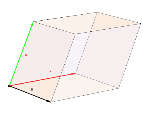
A parallelepiped determined by three vectors u, v, and w consists of the set of points of the form

$r{\bf u} + s{\bf v} + t{\bf w} ,$ where r, s, t are real numbers between 0 and 1, inclusive. The parallelepiped is a 3-dimensional body bounded by parallelograms as shown in the following picture.

ill2 = {Opacity[1, Black], PointSize[Large], Point[p], Arrowheads[Medium], Thick, Black, Arrow[{p, u}], Red, Arrow[{p, v}], Green, Arrow[{p, w}]}; paraP1 = Labeled[Graphics3D[{Opacity[0.2], Parallelepiped[p, {u, v, w}], ill2}, Axes -> False, Boxed -> False, Epilog -> {Text["u", {.15, .22}], Red, Text["v", {.3, .37}], Text["w", {.1, .5}]}], "Parallelepiped", LabelStyle -> FontFamily -> "Times"]

Since the base of the parallelepiped is the parallelogram determined by the vectors u and v, we find is volume, which cross product u × v, as the product of the area and the height, which is projection of ∥ w ∥ on the perpendicular line:

\[Theta] = VectorAngle[w, Cross[u, v]]; arc = ParametricPlot3D[ 1/4 (1/Sqrt[2] (Cos[t]) w + (Sin[t]) Cross[u, v]), {t, 0, Pi/2}, PlotStyle -> Directive[Thick, Black], Boxed -> False, Axes -> False]; ill3 = {Opacity[1, Black], PointSize[Large], Point[p], Arrowheads[Medium], Thick, Black, Arrow[{p, u}], Red, Arrow[{p, v}], Green, Arrow[{p, w}], Blue, Arrow[{p, Cross[u, v]}]}; paraP2 = Manipulate[Labeled[ Show[ Graphics3D[{Opacity[op, Hue[h/3]], Parallelepiped[p, {u, v, w}], ill3}, Axes -> False, Boxed -> False, Epilog -> {Text["\[Theta]", {.070, .35}], Text["u", {.15, .22}], Red, Text["v", {.3, .37}], Text["w", {.18, .7}], Blue, Text["u\[Cross]v", {.07, .5}]} ], arc, BoxRatios -> Automatic] , "Parallelepiped", LabelStyle -> FontFamily -> "Times"], {{op, .156, "Opacity"}, 0, 1, Appearance -> "Labeled"}, {{h, .148, "Hue"}, 0, 1, Appearance -> "Labeled"} ]

p = {0, 0, 0}; {u, v, w} = {{1, 0, 0}, {1, 1, 0}, {0, 1, 1}}; \[Theta] = VectorAngle[w, Cross[u, v]]; arc = ParametricPlot3D[ 1/4 (1/Sqrt[2] (Cos[t]) w + (Sin[t]) Cross[u, v]), {t, 0, Pi/2}, PlotStyle -> Directive[Thick, Black], Boxed -> False, Axes -> False]; ill3 = {Opacity[1, Black], PointSize[Large], Point[p], Arrowheads[Medium], Thick, Black, Arrow[{p, u}], Red, Arrow[{p, v}], Green, Arrow[{p, w}], Blue, Arrow[{p, Cross[u, v]}]}; paraP2 = Labeled[Show[ Graphics3D[{Opacity[.156, Hue[.148/3]], Parallelepiped[p, {u, v, w}], ill3}, Axes -> False, Boxed -> False, Epilog -> {Text["\[Theta]", {.070, .35}], Text["u", {.15, .22}], Red, Text["v", {.3, .37}], Text["w", {.18, .7}], Blue, Text["u\[Cross]v", {.07, .5}]}], arc, BoxRatios -> Automatic], "Figure 9: Parallelepiped", LabelStyle -> FontFamily -> "Times"]

Therefore, we get the volume of the parallelepiped as

$V = \| {\bf u} \times {\bf v} \| \cdot \| {\bf w} \| \,\cos\theta = \left( {\bf u} \times {\bf v} \right) \bullet {\bf w} ,$

where middle dot stands for multiplication of real numbers and • denoted the dot product.

vol = Norm[Cross[u, v]] Norm[w] Cos[\[Theta]]

Also

Cross[u, v] . w

This expression is known as the box product.

Clear[p, u, v, w, \[Theta]]; p = {0, 0, 0}; {u, v, w} = {{1, 0, 0}, {1, 1, 0}, {0, 1, 1}}; \[Theta] = VectorAngle[w, Cross[u, v]]; arc = ParametricPlot3D[ 1/4 (1/Sqrt[2] (Cos[t]) w + (Sin[t]) Cross[u, v]), {t, 0, Pi/2}, PlotStyle -> Directive[Thick, Black], Boxed -> False, Axes -> False]; ill3 = {Opacity[1, Black], PointSize[Large], Point[p], Arrowheads[Medium], Thick, Black, Arrow[{p, u}], Red, Arrow[{p, v}], Green, Arrow[{p, w}], Blue, Arrow[{p, Cross[u, v]}]}; paraP2 = Manipulate[Labeled[ Show[ Graphics3D[{Hue[h, s, b, a], Parallelepiped[p, {u, v, w}], ill3}, Axes -> False, Boxed -> False, Epilog -> {Text["\[Theta]", {.070, .35}], Text["u", {.15, .22}], Red, Text["v", {.3, .37}], Text["w", {.18, .7}], Blue, Text["u\[Cross]v", {.07, .5}]} ], arc, BoxRatios -> Automatic] , "Parallelepiped", LabelStyle -> FontFamily -> "Times"], {{h, .69, "Hue"}, 0, 1, Appearance -> "Labeled"}, {{s, .44, "Saturation"}, 0, 1, Appearance -> "Labeled"}, {{b, .73, "Brightness"}, 0, 1, Appearance -> "Labeled"}, {{a, .5, "Opacity"}, 0, 1, Appearance -> "Labeled"} ]

Theorem 5: Let a, b, and c be three vectors in ℝ³ that define a parallelepiped. The box product (a × b) • c is equal to:

the volume of the parallelepiped, if a, b, and c form a right-handed system;
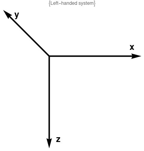
the negative of the volume of the parallelepiped, if a, b, and c form a Left-handed system.

In any case, the volume of the parallelepiped can be computed as the absolute value of the box product, given by |(a × b) • c|.

Corollary 1: The box product (a × b) • c is

positive, if a, b, and c form a right-handed system;
negative, if a, b, and c form a left-handed system;
zero, if a, b, and c are coplanar.

Example 4: From the definition of the vector product, it follows that

$\left\vert {\bf a} \times {\bf b} \right\vert = \mbox{ area of the parallelogram defined by} \quad {\bf a} \mbox{ and } {\bf b} .$

So we can use Eq.

$\eqref{EqCross.6}$ to find the area of a parallelogram defined by two vectors directly in terms of their components. For instance, the area defined by a = (1, −1, 2) and b = (−2, 3, 1) can be found by calculating their vector product

${\bf a} \times {\bf b} = \det \begin{bmatrix} \hat{\bf e}_1 & \hat{\bf e}_2 & \hat{\bf e}_3 \\ 1 & -1 & 2 \\ -2 & 3 & 1 \end{bmatrix} = -7\,{\bf i} -5\,{\bf j} + {\bf k}$

Cross[{1,-1,2}, {-2,3,1}]

{-7, -5, 1}

Its absolute value is approximately 8.66025 .

$\| (-7,-5,1) \| = \sqrt{7^2 + 5^2 + 1} = \sqrt{49 + 26} = \sqrt{75} = 5\sqrt{3} \approx 8.66025 .$

Norm[%]

5 Sqrt[3]

End of Example 4

■

Example 5: The volume of a parallelepiped defined by three non-coplanar vectors a, b, and c is given by

$\displaystyle \left\vert {\bf a} \bullet \left( {\bf b} \times {\bf c} \right) \right\vert .$ The absolute value is taken to ensure the positivity of the area. In terms of components we have

$\mbox{volume} = \left\vert \det \begin{bmatrix} \alpha_1 & \alpha_2 & \alpha_3 \\ \beta_1 & \beta_2 & \beta_3 \\ \gamma_1 & \gamma _2 & \gamma_3 \end{bmatrix} \right\vert .$

Taking three vectors a = (1,2,-3), b = (4, -2, 1), and c = (2, -1,-5), we find

$\mbox{volume} = \left\vert \det \begin{bmatrix} 1 & \phantom{-}2 & -3 \\ 4 & -2 & \phantom{-}1 \\ 2 & -1 & -5 \end{bmatrix} \right\vert = 55.$

Det[{{1,2,-3},{4,-2,1},{2,-1,-5}}]

End of Example 5

■

Example 6: Which of the following systems of vectors u, v, w is right-handed? Which one is left-handed? Which one is coplanar?

[1, 2, 0], [0, 1, 1], [1, -1, 1]
[0, 1,2], [-1,2,2], 0, 1, 1]
[1, 1, 2], [1, 2, 2], [0, 1, 1]

Solution: When the Box Product (Cross[u, v].w) is positive, the system is right handed; negative, left handed; zero, coplanar, thus, entering a system into the following function as a list of lists, we have:

box[system_ : List] := If[Cross[system[[1]], system[[2]]] . system[[3]] > 0, Print["The system is right handed"], If[Cross[system[[1]], system[[2]]] . system[[3]] < 0, Print["The system is left handed"], Print["The system is coplanar"]]];

box[{{1, 2, 0}, {0, 1, 1}, {1, -1, 1}}]

The system is right handed

box[{{1, 1, 2}, {1, 2, 3}, {0, 1, 1}}]

The system is coplanar

box[{{0, 1, 2}, {-1, 2, 2}, {0, 1, 1}}]

The system is left handed

End of Example 6

■

Theorem 6: Let a and b be two vectors in ℝ³. Then (a × b) • c = a • (b × c).

This follows from observing that both (a × b) • c and a • (b × c) compute the same box product, i.e., they either both give the volume of the parallelepiped or they both give the negative of the volume.

Alternatively, we can calculate each product explicitly: $\begin{align*} \left( {\bf u} \times {\bf v} \right) \bullet {\bf w} &= u_2 v_3 w_1 - u_3 v_2 w_1 + u_3 v_1 w_2 - u_1 v_3 w_2 + u_1 v_2 w_3 - u_2 v_1 w_3 , \\ {\bf u} \bullet \left( {\bf v} \times {\bf w} \right) &= u_2 v_3 w_1 - u_3 v_2 w_1 + u_3 v_1 w_2 - u_1 v_3 w_2 + u_1 v_2 w_3 - u_2 v_1 w_3 . \end{align*}$

Coordinates are “functions” that specify points of a space. The smallest number of these functions necessary to specify a point P is called the dimension of that space. There are three widely used orthogonal coordinate systems in a three-dimensional vector space ℝ³: Cartesian (x(P), y(P), z(P)), cylindrical (r(P), θ(P), z(P)), and spherical (ρ(P), θ(P), φ(P)). The latter φ(P) is called the azimuth or the azimuthal angle of P, while θ(P) is called its polar angle.

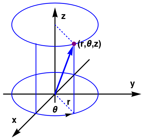
Cylindrical coordinates

A cylindrical coordinate system in ℝ³ is a marriage of polar coordinates on the plane ℝ² and regular applicate direction from the Cartesian one. A cylindrical coordinates (r ≥ 0, 0 ≤ θ < 2π, −∞ < z < ∞) of a point in ℝ³ are defined by the equations:

$\begin{split} x &= r\,\cos\theta , \\ y &= r\,\sin\theta , \\ z &= z , \end{split} \qquad\quad r = +\sqrt{x^2 + y^2} , \qquad \theta = \begin{cases} \arctan\left( \frac{y}{x} \right) , & \quad \mox{if } x > 0, \\ \arctan\left( \frac{y}{x} \right) + \pi , & \quad \mbox{if } x < 0 \mbox{ and } y \ge 0 , \\ \arctan\left( \frac{y}{x} \right) - \pi , & \quad \mbox{if } x < 0 \mbox{ and } y < 0, \\ \frac{pi}{2} \cdot \frac{y}{|y|} , & \quad \mbox{if } x = 0 \mbox{ and } y \ne 0 , \\ \mbox{indetermined} , & \quad \mbox{if } x= 0 \mbox{ and } y = 0. \end{cases}$

ii = Graphics[{Arrowheads[0.07], Thickness[0.007], Arrow[{{0.4, 0.4}, {-0.5, -0.5}}]}]; jj = Graphics[{Arrowheads[0.07], Thickness[0.007], Arrow[{{-0.6, 0}, {1, 0}}]}]; kk = Graphics[{Arrowheads[0.07], Thickness[0.007], Arrow[{{0, -0.1}, {0, 1}}]}]; ti = Graphics[Text[Style["x", Bold, FontSize -> 22], {-0.47, -0.3}]]; tj = Graphics[Text[Style["y", Bold, FontSize -> 22], {0.9, 0.12}]]; tk = Graphics[ Text[Style["z", Bold, FontSize -> 22], {0.1, 0.9}]]; circle = Graphics[{Blue, Thick, Circle[{0, 0}, {0.5, 0.25}]}]; circle2 = Graphics[{Blue, Thick, Circle[{0, 0.8}, {0.5, 0.25}]}]; line1 = Graphics[{Blue, Thick, Line[{{-0.22, -0.22}, {-0.22, 0.58}}]}]; line2 = Graphics[{Blue, Thick, Line[{{0.22, -0.22}, {0.22, 0.58}}]}]; line3 = Graphics[{Blue, Thick, Dashed, Line[{{0.22, -0.22}, {0, 0}}]}]; line4 = Graphics[{Blue, Thick, Dashed, Line[{{0.22, 0.58}, {0, 0.8}}]}]; tr = Graphics[ Text[Style["r", Bold, FontSize -> 22], {0.16, -0.09}]]; tt = Graphics[ Text[Style["\[Theta]", Bold, FontSize -> 22], {0., -0.18}]]; tz = Graphics[ Text[Style["(r,\[Theta],z)", Bold, FontSize -> 22], {0.4, 0.58}]]; disk = Graphics[{Purple, Disk[{0.22, 0.58}, 0.025]}]; ar = Graphics[{Blue,Arrowheads[0.07], Thickness[0.01], Arrow[{{0, 0}, {0.21, 0.56}}]}]; Labeled[ arr = Graphics[{Arrowheads[0.05], Thickness[0.01], Arrow[{{0.15, -0.238}, {0.2, -0.227}}]}]; Labeled[Show[ii, jj, kk, ti, tj, tk, circle, circle2, line1, line2, line3, line4, tr, tt, tz, disk, ar,arr], "Figure10: Cylindrical coordinates"]

Variable r is the radius of the cylinder passing through point P(r, θ, z) or the radial distance distance from the applicate (z-axis); θ is called azimuthal angle and it is measured from the abscissa (x-axis) in the xy-plane, and z is the same as in the Cartesian system. A vector v (with endpoint P) in cylindrical coordinates can be written as

${\bf v} = v_r \hat{\bf r}(\theta ) + v_z \hat{\bf z} ,$

where

$\displaystyle \hat{\bf r}, \ \hat{\theta}, \ \hat{\bf z}$ are nit vectors in r, θ, and z directions, respectively. They are pointed in direction of increasing of corresponding coordinates. Note that the radial unit vector

$\displaystyle \hat{\bf r} (\theta )$ depends on angle θ.

The unit vectors in the cylindrical coordinate system are functions of position. It is convenient to express them in terms of unit vectors of the rectangular coordinate system that are not themselves functions of position.

$\hat{\bf r} = \begin{pmatrix} \cos\theta \\ \sin\theta \\ 0 \end{pmatrix} , \qquad \hat{\theta} = \begin{pmatrix} -\sin\theta \\ \cos\theta \\ 0 \end{pmatrix} , \qquad \hat{\bf z} = \begin{pmatrix} 0 \\ 0 \\ 1 \end{pmatrix} ,$

$\begin{split} \hat{r} &= \hat{\bf x}\,\cos\theta + \hat{\bf y}\,\sin\theta , \\ \hat{\theta} &= -\hat{\bf x}\,\sin\theta + \hat{\bf y} \,\cos\theta , \\ \hat{\bf z} &= \hat{\bf z} . \end{split}$

Here

$\displaystyle \hat{\bf x} = {\bf i}, \ \hat{\bf y} = {\bf j}, \ \hat{\bf z} = {\bf k}$ are unit vectors in Cartesian coordinates. The inverse formulas are

$\begin{split} \hat{\bf x} &= {\bf i} = \hat{r}\,\cos\theta - \hat{\theta} \sin\theta , \\ \hat{\bf y} &= {\bf j} = \hat{r} \sin\theta + \hat{\theta} \cos\theta , \\ \hat{\bf z} &= {\bf k} = \hat{\bf z} . \end{split}$

Clear[t]; Solve[{rr == x*Cos[t] + y*Sin[t], tt == -x*Sin[t] + y*Cos[t]}, {x, y}]; FullSimplify[%]

{x -> rr Cos[t] - tt Sin[t], y -> tt Cos[t] + rr Sin[t]}}

The position vector r of a point in terms of unit vectors is

${\bf r} = x\,\hat{\bf x} + y\,\hat{\bf y} + z\,\hat{\bf z} = r\,\hat{\bf r} + z\,\hat{\bf z} .$

Cross products of the utit vectors in cylindrical coordinates show that they are orthogonal

$\begin{split} \hat{\bf r} \times \hat{\bf z} &= -\hat{\theta} , \\ \hat{\theta} \times \hat{\bf z} &= \hat{\bf r} , \\ \hat{\bf r} \times \hat{\theta} &= \hat{\bf z} . \end{split}$

Cross product of two vectors written in cylindrical coordinates is expressed in Cartesian coordinates as

$\begin{equation} \label{EqCross.7} \begin{bmatrix} r_1 \\ \theta_1 \\ z_1 \end{bmatrix} \,\times \, \begin{bmatrix} r_2 \\ \theta_2 \\ z_2 \end{bmatrix} = \left[ \begin{array}{c} z_2 r_1 \sin\theta_1 - z_1 r_2 \sin\theta_2 \\ z_1 r_2 \cos\theta_2 - z_2 r_1 \cos\theta_1 \\ r_1 r_2 \,\sin \left( \theta_2 - \theta_1 \right) \end{array} \right] . \end{equation}$

In cylindrical coordinates, we have

$\left( r_1\,\hat{\bf r}_1 + z_1\,\hat{\bf z} \right) \times \left( r_2\,\hat{\bf r}_2 + z_2\,\hat{\bf z} \right) = r_1 r_2 \hat{\bf r} (\theta_1) \times \hat{\bf r} (\theta_2 ) + \left( r_2 z_1 - r_1 z_2 \right) \hat{\theta} ,$

where

$\displaystyle \hat{\bf r}_1 = \hat{\bf r} (\theta_1 )$ is the unit radial vector for point (r₁ , θ₁) and

$\displaystyle \hat{\bf r}_2 = \hat{\bf r} (\theta_2 )$ is the unit radial vector towards point (r₂ , θ₂). These radial vectors are applied at two different points, so their cross product has no natural (simple) way to be specified.

The gradient operator in cylindrical coordinates is given by

$\nabla = \hat{\bf r} \,\frac{\partial}{\partial r} + \hat{\theta} \,\frac{1}{r}\,\frac{\partial}{\partial \theta} + \hat{\bf z}\,\frac{\partial}{\partial z} .$

Example 7: Let us consider two vectors (for simplicity, written in column form)

${\bf a} = \begin{pmatrix} 1 \\ 2 \\ 2 \end{pmatrix} \qquad\mbox{and} \qquad {\bf b} = \begin{pmatrix} \phantom{-}2 \\ -2 \\ -1 \end{pmatrix} .$ Their cross product is

${\bf a} \times {\bf b} = \begin{pmatrix} 1 \\ 2 \\ 2 \end{pmatrix} \times \begin{pmatrix} \phantom{-}2 \\ -2 \\ -1 \end{pmatrix} = \begin{pmatrix} \phantom{-}2 \\ \phantom{-}5 \\ -6 \end{pmatrix} .$

Cross[{1, 2, 2}, {2, -2, -1}]

{2, 5, -6}

Now we rewrite these vectors into cylindrical coordinate system

${\bf a} = \left(\sqrt{5}, \theta_1 , 2 \right) , \qquad {\bf b} = \left( \sqrt{8}, \theta_2 , -1 \right) , \qquad {\bf a} \times {\bf b} = \left( \sqrt{29} , \theta_3 , -6 \right) ,$ where

$\theta_1 = \arctan \left( 2 \right) \approx 1.10715 , \qquad \theta_2 = 2\pi - \frac{\pi}{4} = \frac{7\pi}{4} \approx 5.49779 , \qquad \theta_3 = \arctan \left( \frac{5}{2} \right) \approx 1.19029 .$

N[ArcTan[2]]

1.10715

N[ArcTan[5/2]]

1.19028994968253102899496825317

First, we verify cylindrical coordinates of these three vectors with formulas:

$\begin{align*} r_a &= 1\cdot \cos \theta_1 + 2\cdot \sin\theta_1 \approx 2.23607 \approx \sqrt{5} , \\ r_b &= 2 \cdot \cos \theta_2 - 2\cdot \sin\theta_2 \approx 2.82843 \approx \sqrt{8} , \\ r_{ab} &= 2 \cdot \cos \theta_3 + 5\cdot \sin\theta_3 \approx 5.38516 \approx \sqrt{29} . \end{align*}$

t1 = N[ArcTan[2]];
Cos[t1] + 2*Sin[t1]

2.23606797749979

N[Sqrt[5]]

2.23606797749979

t2 = 2*Pi -Pi/4 ; 2*Cos[t2] - 2*Sin[t2]

2 Sqrt[2]

N[Sqrt[8]]

2.82843

t3 = N[ArcTan[5/2]]; 2*Cos[t3] + 5*Sin[t3]

5.38516

N[Sqrt[29]]

5.385164807134504

Using vector notation, we have

${\bf a} = \sqrt{5}\,\hat{\bf r} + 2\,\hat{\bf z} , \qquad {\bf b} = 2\sqrt{2}\,\hat{\bf r} - \hat{\bf z} , \qquad {\bf a} \times {\bf b} = \sqrt{29}\, \hat{\bf r} - 6\,\hat{\bf z} .$ Then we find their cross product using Eq.(7).

${\bf a} \times {\bf b} = \left[ \begin{array}{c} z_2 r_1 \sin\theta_1 - z_1 r_2 \sin\theta_2 \\ z_1 r_2 \cos\theta_2 - z_2 r_1 \cos\theta_1 \\ r_1 r_2 \,\sin \left( \theta_2 - \theta_1 \right) \end{array} \right] = \left[ \begin{array}{c} (-1)\cdot \sqrt{5}\cdot \sin\theta_1 - 2 \cdot \sqrt{8} \cdot \sin\theta_2 \\ 2\cdot \sqrt{8} \cdot cos\theta_2 - (-1)\cdot \sqrt{5}\cdot \cos \theta_2 \\ \sqrt{5} \cdot \sqrt{8}\cdot \sin\left( \theta_2 - \theta_1 \right) \end{array} \right] ,$ which we simplify to

${\bf a} \times {\bf b} = \left[ \begin{array}{c} 2. \\ 5. \\ -6. \end{array} \right] .$

(-1)*Sqrt[5]*Sin[t1] - 2*Sqrt[8]*Sin[t2]

Sqrt[8]*Cos[t2] + Sqrt[5]*Cos[t1]

Sqrt[5]*Sqrt[8]*Sin[t2 - t1]

-6.

End of Example 7

■

Spherical coordinates

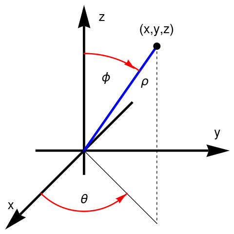
A spherical coordinate system is a coordinate system for three-dimensional space ℝ³, where the position of a point is specified by three numbers: the radial distance of that point from a fixed origin; its zenith angle (or inclination angle or polar angle) measured from an applicat direction; and the azimuthal angle of its orthogonal projection on a reference plane that passes through the origin and is orthogonal to the fixed axis, measured from another fixed reference direction on that plane. The spherical coordinates (ρ, θ, ϕ) are related to the Cartesian coordinates (x, y, z) by

$\begin{split} x &= \rho\,\cos\theta\,\sin\phi , \\ y &= \rho\,\sin\theta \,\sin\phi , \\ z &= \rho\,\cos\phi , \end{split} \qquad \rho \geqslant 0, \quad \theta \in [0, 2\pi ), \quad \phi \in [0, \pi ] ,$

where the radial, azimuth, and zenith angle coordinates are taken as ρ, θ, and ϕ, respectively. As usual, the location of a point (x, y, z) is specified by the distance ρ of the point from the origin, the angle ϕ between the position vector and the z-axis, the polar angle measured down from the north pole, and the azimuthal angle θ from the x-axis to the projection of the position vector onto the xy plane, analogous to longitude in earth measuring coordinates:

$\rho = \sqrt{x^2 + y^2 + z^2} \geqslant 0 \qquad\mbox{and} \qquad \phi = \mbox{arccos} \frac{z}{\rho} = \begin{cases} \arctan \frac{\sqrt{x^2 + y^2}}{z} , & \mbox{ if } z > 0, \\ \pi + \arctan \frac{\sqrt{x^2 + y^2}}{z} , & \mbox{ if } z < 0, \\ + \frac{\pi}{2} , & \mbox{ if } z = 0 \mbox{ and } xy \ne 0 , \\ \mbox{undefined} , & \mbox{ i } x=y=z=0 . \end{cases}$

While zenith angle is take from the closed interval 0 ≤ ϕ ≤ π, the azimuth angle belongs to semiclosed interval 0 ≤ θ < 2π.

$\theta = \mbox{sign}(y)\,\arccos \frac{x}{\sqrt{x^2 + y^2}} = \begin{cases} \arctan \left( y/x \right) , & \ \mbox{ if} \quad x > 0 , \\ \arctan \left( y/x \right) + \pi , & \ \mbox{ if} \quad x < 0 \mbox{ and } y \ge 0, \\ \arctan \left( y/x \right) - \pi , & \ \mbox{ if} \quad x < 0 \mbox{ and } y < 0, \\ +\frac{\pi}{2} , & \ \mbox{ if} \quad x = 0 \mbox{ and } y > 0, \\ -\frac{\pi}{2} , & \ \mbox{ if} \quad x = 0 \mbox{ and } y < 0, \\ \mbox{undefined}, & \ \mbox{ if} \quad x = 0 \mbox{ and } y=0. \end{cases} .$

		az = Graphics[{Black, Thickness[0.01], Arrowheads[0.1], Arrow[{{0, -0.2}, {0, 1.2}}]}]; ax = Graphics[{Black, Thickness[0.01], Arrowheads[0.1], Arrow[{{0.4, 0}, {-0.65, -0.65}}]}]; ay = Graphics[{Black, Thickness[0.01], Arrowheads[0.1], Arrow[{{-0.4, 0}, {1.2, 0}}]}]; line = Graphics[{Blue, Thickness[0.01], Line[{{0, 0}, {0.6, 0.86}}]}]; line1 = Graphics[{Black, Dashed, Line[{{0.6, 0.86}, {0.6, -0.6}}]}]; line2 = Graphics[{Black, Line[{{0, 0}, {0.6, -0.6}}]}]; circle1 = Graphics[{Red, Thick, Circle[{0, 0}, 0.8, {Pi/2, 0.97}]}]; circle2 = Graphics[{Red, Thick, Circle[{0, 0}, 0.5, {-Pi/4, -3*Pi/4}]}]; ar1 = Graphics[{Red, Arrowheads[0.05], Arrow[{{0.36, 0.72}, {0.42, 0.67}}]}]; ar2 = Graphics[{Red, Arrowheads[0.05], Arrow[{{0.3, -0.395}, {0.35, -0.355}}]}]; disk = Graphics[Disk[{0.6, 0.86}, 0.03]]; tx = Graphics[{Black, Text[Style["x", 20], {-0.6, -0.45}]}]; ty = Graphics[{Black, Text[Style["y", 20], {1.1, 0.15}]}]; tz = Graphics[{Black, Text[Style["z", 20], {0.15, 1.1}]}]; tf = Graphics[{Black, Text[Style[\[Phi], 20], {0.18, 0.6}]}]; tt = Graphics[{Black, Text[Style[\[Theta], 20], {0, -0.4}]}]; tp = Graphics[{Black, Text[Style["(x,y,z)", 20], {0.6, 1.0}]}]; tr = Graphics[{Black, Text[Style[\[Rho], 20], {0.5, 0.57}]}]; Labeled[Show[ax, ay, az, line, line1, line2, circle1, circle2, ar1, ar2, disk, tx, ty, tz, tf, tt, tp, tr], "Spherical Coordinates"]
Spherical coordinates.		Mathematica code

Unit vectors in spherical coordinates are

$\hat{\rho} = \begin{pmatrix} \cos\theta\,\sin\phi \\ \sin\theta \,\sin\phi \\ \cos\phi \end{pmatrix} , \qquad \hat{\theta} = \begin{pmatrix} -\sin\theta \\ \cos\theta \\ 0 \end{pmatrix} , \qquad \hat{\phi} = \begin{pmatrix} \cos\theta \,\cos\phi \\ \sin\theta \,\cos\phi \\ -\sin\phi \end{pmatrix} .$

They can be expressed through Cartesian unit vectors as follows:

$\begin{split} \hat{\rho} &= \cos\theta\,\sin\phi \,\hat{\bf x} + \sin\theta \,\sin\phi \,\hat{\bf y} + \cos\phi\,\hat{\bf z} , \\ \hat{\theta} &= -\sin\theta \,\hat{\bf x} + \cos\theta \,\hat{\bf y} , \\ \hat{\phi} &= \cos\theta\,\cos\phi\,\hat{\bf x} + \sin\theta \,\cos\phi\,\hat{\bf y} -\sin\phi\,\hat{\bf z} , \end{split}$

and

$\begin{split} \hat{\bf x} &= {\bf i} = \cos\theta\,\sin\phi\,\hat{\rho} + \sin\theta\, \hat{\theta} + \cos\theta\, \cos\phi\,\hat{\phi} , \\ \hat{\bf y} &= {\bf j} = \sin\theta\,\sin\phi\,\hat{\rho} + \cos\theta \,\hat{\theta} + \sin\theta\,\cos\phi\, \hat{\phi} , \\ \hat{\bf z} &= {\bf k} = \cos\phi\,\hat{\rho} - \sin\phi\,\hat{\phi} . \end{split}$

Solve[{rr == Sin[\[Phi]]*Cos[\[Theta]]*x + Sin[\[Phi]]*Sin[\[Theta]]*y + Cos[\[Phi]]*z, pp == Cos[\[Phi]]*Cos[\[Theta]]*x + Cos[\[Phi]]*Sin[\[Theta]]*y - Sin[\[Phi]]*z, tt == -Sin[\[Theta]]*x + Cos[\[Theta]]*y}, { x, y, z}]Solve[{rr == Sin[\[Phi]]*Cos[\[Theta]]*x + Sin[\[Phi]]*Sin[\[Theta]]*y + Cos[\[Phi]]*z, pp == Cos[\[Phi]]*Cos[\[Theta]]*x + Cos[\[Phi]]*Sin[\[Theta]]*y - Sin[\[Phi]]*z, tt == -Sin[\[Theta]]*x + Cos[\[Theta]]*y}, { x, y, z}]

FullSimplify[%];
TableForm[Transpose[%]]

{{x -> -tt Sin[\[Theta]] + Cos[\[Theta]] (pp Cos[\[Phi]] + rr Sin[\[Phi]]), y -> Cos[\[Theta]] (tt + pp Cos[\[Phi]] Tan[\[Theta]] + rr Sin[\[Phi]] Tan[\[Theta]]), z -> rr Cos[\[Phi]] - pp Sin[\[Phi]]}}

A position vector in spherical coordinates is described in terms of the radial parameters ρ, which depends on the zenith (or polar) angle ϕ and the azimuthal angle θ as follows:

${\bf r} = \rho\,\hat{\rho} (\theta , \phi ) .$

The cross product of unit vectors in spherical coordinates is given by the rule (which shows that they are orthogonal):

$\begin{equation} \label{EqCross.8} \begin{split} \hat{\rho} \times \hat{\theta} &= \hat{\phi} , \\ \hat{\rho} \times \hat{\phi} &= -\hat{\theta} , \\ \hat{\theta} \times \hat{\phi} &= \hat{\rho} . \end{split} \end{equation}$

However, these formulas are of little help for determinantion of cross product in spherical coordinates because unit vectors depend on location of the given two vectors. Therefore, the rules above are not directly applicable for cross product.

Suppose that two vectors are given in Cartesian and spherical coordinates

${\bf a} = \begin{pmatrix} a_x \\ a_y \\ a_z \end{pmatrix} = \begin{pmatrix} \rho_a \cos\theta_a \sin\phi_a \\ \rho_a \sin\theta_a \sin\phi_a \\ \rho_a \cos\phi_a \end{pmatrix} \qquad \mbox{and} \qquad {\bf b} = \begin{pmatrix} b_x \\ b_y \\ b_z \end{pmatrix} = \begin{pmatrix} \rho_b \cos\theta_b \sin\phi_b \\ \rho_b \sin\theta_b \sin\phi_b \\ \rho_b \cos\phi_b \end{pmatrix} .$

The radial distance ρ_ab of their cross product a × b is known to be

$\rho_{ab} = \| {\bf a} \| \cdot \| {\bf b} \| \,\sin\alpha = \rho_a \rho_b \sin\alpha ,$

where α is the angle between these two given vectors. Its value can be determined from their dot product:

$\cos \alpha = \frac{{\bf a} \bullet {\bf b}}{\| {\bf a} \| \cdot \| {\bf b} \|} = \frac{{\bf a} \bullet {\bf b}}{\rho_a \cdot \rho_b} .$

Using expressions of Cartesian components via spherical coordinates, we find

${\bf a} \bullet {\bf b} = \rho_a \rho_b \left[ \cos\theta_a \,\sin\phi_a \,\cos\theta_b \,\sin\phi_b + \sin\theta_a\,\sin \phi_a \,\sin\theta_b \,\sin\phi_b + \cos\phi_a \,\cos\phi_b \right] .$

With the aid of trigonometric identity cosα cosβ + sinα sinβ = cos(α − β), we slightly simplify the expression

$\sin\alpha = \sqrt{1 - \left[ \sin\phi_a \,\sin\phi_b \,\cos \left( \theta_a - \theta_b \right) + \cos\phi_a \,\cos\phi_b \right]^2} ,$

which resembles the formula

$\sin\alpha = \sqrt{1 - \cos^2 \alpha} .$

This allows us determine the components of cross product:

$\begin{align*} {\bf a} \times {\bf b} &= \rho_a \rho_b \begin{pmatrix} \left( \sin\theta_a \sin\phi_a \right) \left( \cos\phi_b \right) - \left( \sin\theta_b \sin\phi_b \right) \left( \cos\phi_a \right) \\ \cos \phi_a \left( \cos\theta_b \sin\phi_b \right) - \cos \phi_b \left( \cos\theta_a \sin\phi_a \right) \\ \left( \cos\theta_a \sin\phi_a \right) \left( \sin\theta_b \sin\phi_b \right) /\sin\alpha - \left( \cos\theta_b \sin\phi_b \right) \left( \sin\theta_a \sin\phi_a \right) /\sin\alpha \end{pmatrix} \\ &= \rho_a \rho_b \begin{pmatrix} \sin\theta_a \sin\phi_a \, \cos\phi_b - \sin\theta_b \sin\phi_b \, \cos\phi_a \\ \cos \phi_a \left( \cos\theta_b \sin\phi_b \right) - \cos \phi_b \left( \cos\theta_a \sin\phi_a \right) \\ \sin\phi_a \sin \phi_b \sin \left( \theta_b - \theta_a \right) /\sin\alpha \end{pmatrix} \tag{8} \\ &= \begin{bmatrix} \rho = \rho_a \rho_b \sqrt{1 - \left[ \sin\phi_a \,\sin\phi_b \,\cos \left( \theta_a - \theta_b \right) + \varepsilon\,\cos\phi_a \,\cos\phi_b \right]^2} \\ \theta = \mbox{not available} \\ \phi = \arccos \left\{ \sin\phi_a \sin \phi_b \sin \left( \theta_b - \theta_a \right) /\sin\alpha \right\} \end{bmatrix} , \tag{8a} \end{align*}$

where ε takes care of signs of cosines of angles ϕ_a and ϕ_b.

The gradient in spherical coordinates is

$\nabla = \hat{\rho}\,\frac{\partial}{\partial \rho} + \frac{1}{\rho}\,\hat{\phi}\,\frac{\partial}{\partial\phi} + \frac{1}{\rho\,\sin\phi} \,\hat{\theta}\,\frac{\partial}{\partial\theta} .$

Example 8: We reconsider the previous example and consider the same two vectors

${\bf a} = \begin{pmatrix} 1 \\ 2 \\ 2 \end{pmatrix} = \begin{bmatrix} 3 \\ \theta_a \\ \phi_a \end{bmatrix} , \qquad {\bf b} = \begin{pmatrix} \phantom{-}2 \\ -2 \\ -1 \end{pmatrix} = \begin{bmatrix} 3 \\ \theta_b \\ \phi_b \end{bmatrix} ,$ where

$\theta_a = \arctan (2) \approx 1.10715 , \quad \phi_a = \arctan \left( \frac{\sqrt{5}}{2} \right) \approx 0.841069 , \qquad \theta_b = \frac{7\pi}{4} \approx 5.49779 , \quad \phi_b = \pi - \arctan \left( 2\sqrt{2} \right) \approx 1.91063 .$ We recalculate the spherical coordinates of their cross product using Eq.(8) and Eq.(8a).

${\bf a} \times {\bf b} = \begin{pmatrix} \phantom{-}2 \\ \phantom{-}5 \\ -6 \end{pmatrix} = \begin{bmatrix} \rho_{ab} \\ \theta_{ab} \\ \phi_{ab} \end{bmatrix} ,$ where

$\begin{align*} \rho_{ab} &= \sqrt{2^2 + 5^2 + 6^2} = \sqrt{65} = \rho_a \cdot \rho_b \,\sin\alpha \approx 8.06226 , \\ \theta_{ab} &= \arctan \left( \frac{5}{2} \right) \approx 1.19029 \\ \phi_{ab} &= \pi - \arctan \left( \frac{\sqrt{29}}{6} \right) \approx 2.4101452723348746 . \end{align*}$

r=N[Sqrt[4 + 25 + 36]]

8.06226

t1 = N[ArcTan[2]];
p1 = N[ArcTan[Sqrt[5]/2]];
t2 = 7*Pi/4;
p2 = N[ArcTan[Sqrt[8]]];
tab = N[ArcTan[5/2]] ;
pab = N[Pi - ArcTan[Sqrt[29]/6]];
3*Cos[t1]*Sin[p1]

3*Cos[t2]*Sin[p2]

r*Cos[tab]*Sin[pab]

Now we check the value of sine of angle between these two vectors:

$\cos \alpha = \frac{{\bf a} \bullet {\bf b}}{\| {\bf a} \| \cdot \| {\bf b} \|} = \frac{{\bf a} \bullet {\bf b}}{\rho_a \cdot \rho_b} = \frac{-4}{9} \qquad \Longrightarrow \qquad \sin\alpha = \sqrt{1 - \frac{36}{81}} = \frac{\sqrt{65}}{9} \approx 0.895806 .$

sina = Sqrt[1 - (Sin[p1]*Sin[p2]*Cos[t1 - t2] - Cos[p1]*Cos[p2])^2]

0.895806

As you see, we used minus when evaluated cosine function because z-coordinate of a × b is negative. We compare sin(α) evaluated with trigonometric functions above with the definition followed from Cartesian form:

N[Sqrt[65]/9]

0.895806

We verify formula (8a) for radial distance

9*sina

8.06226

which gives the value √65 ≈ 8.06226. Finally, we check the formula for ϕ_ab

ArcCos[Sin[p1]*Sin[p2]*Sin[t2 - t1]/sina]

2.41015

This value is equal to the "exact" value 2.410 evaluated with the aid of arctangent function.

End of Example 8

■

Mathematica has three multiplication commands for vectors: the dot (or inner) and outer products (for arbitrary vectors), and the cross product (for three dimensional vectors).

The cross product can be done on two vectors. It is important to note that the cross product is an operation that is only functional in three dimensions. The operation can be computed using the Cross[vector 1, vector 2] operation or by generating a cross product operator between two vectors by pressing [Esc] cross [Esc]. ([Esc] refers to the escape button)

Cross[{1,2,7}, {3,4,5}]

{-18,16,-2}

Applications in Physics

The simplest physical model of a vector product is the moment M of a force F about a point 0 (the origin), defined as

${\bf M} = {\bf r} \times {\bf F} ,$

where r is the vector joining the origin to the initial point of F. The positive direction of the vector M depends on the choice of the coordinate system, like the direction of the angular velocity vector due to the action of the moment M.

An electric charge e in an electric field E experiences a force

${\bf F}_e = e\,{\bf E} ,$

while an electric charge e moving with velocity v in a magnetic field H experiences a force

${\bf F}_m = \frac{e}{c} \left( {\bf v} \times {\bf H} \right) ,$

where c is the velocity of light.9 Hence, the total force experienced by an electric charge e moving with velocity v in an electromagnetic field with electric field E and magnetic field H is given by

${\bf F} = e\.{\bf E} + \frac{e}{c} \left( {\bf v} \times {\bf H} \right) .$

If the charge moves a distance dr in time dt, the work done by the electromagnetic field is

${\bf F} \bullet {\text d}{\bf r} = {\bf F} \bullet \frac{{\text d}{\bf r}}{{\text d}t} \,{\text d}t = {\bf F} \bullet {\bf v} \,{\text d} t = \left[ e\.{\bf E} + \frac{e}{c} \left( {\bf v} \times {\bf H} \right) \right] \bullet {\bf v}\,{\text d} t .$

This work goes into changing the kinetic energy U of the moving charge. The magnetic field does no work because the force F_m due to the magnetic field is perpendicular to v at every instant. Hence the work done by the electromagnetic field is due to the electric field alone and is done at the rate

$\frac{{\text d}U}{{\text d}t} = e\,{\bf E} \bullet {\bf v} .$

The magnetic field changes the direction of the charge's velocity, but not the magnitude of the velocity.

Which of the following systems of vectors are right-handed? Which are left-handed? ${\bf a} \quad {\bf k, \ i, \ j}; \qquad {\bf b} \quad$
Show that if a × u = 0, then a = 0.
Find the area of the parallelogram determined by the vectors (1, 2, &mnus;3) and (2, −1, 2).
Find the area of the parallelogram determined by the vectors
Find the area of the triangle determined by the three points
Find the volume of the parallelepiped determined by the vectors
Which of the following systems of three vectors are right-handed? Which are left- handed? Which are coplanar? ${\bf a} \quad$
Suppose you are given three vectors whose components are all integers. Can you conclude the volume of the parallelepiped determined from these three vectors will always be an integer?
Is u × (v × w) = (u × v) × w ? What is the meaning of u × v × w ?
Show by direct computation that $\begin{align*} \| {\bf a} \times {\bf b} \|^2 &= \| {\bf a} \|^2 \| {\bf b} \|^2 - \left( {\bf a} \bullet {\bf b} \right)^2 \\ &= \| {\bf a} \|^2 \| {\bf b} \|^2 \left( 1 - \cos^2 \theta \right) , \end{align*}$ where θ is the angle included between the two vectors.
Prove the identity: ${\bf a} \times ({\bf b} \times {\bf c}) = \left( {\bf a} \bullet {\bf c} \right) {bf b} - \left( {\bf a} \bullet {\bf b} \right) {bf c} .$
Prove the Jacobi identity: ${\bf a} \times ({\bf b} \times {\bf c}) + {\bf b} \times ({\bf c} \times {\bf a}) + {\bf c} \times ({\bf a} \times {\bf b}) = {\bf 0} .$
Show that $\left( {\bf a} \times {\bf b} \right) \bullet {\b c} = \left( {\bf b} \times {\bf c} \right) \bullet {\b a} = \left( {\bf c} \times {\bf a} \right) \bullet {\b b} .$
Show that $\left( {\bf u} \times {\bf v} \right)' = {\bf u}' \times {\bf v} + {\bf u} \times {\bf v}' ,$ where prime stands for the derivative.

Anton, Howard (2005), Elementary Linear Algebra (Applications Version) (9th ed.), Wiley International
Beezer, R.A., A First Course in Linear Algebra, 2017.
Fitzpatrick, S., Linear Algebra: A second course, featuring proofs and Python. 2023.
Selinger, P., Matrix Theory and Linear Algebra,

Introduction to Linear Algebra

Systems of Linear Equations

Matrix Algebra

Vector Spaces

Eigenvalues, Eigenvectors

Euclidean Spaces

Matrix Decompositions

Tensors

Applications

Functions of Matrices

Miscellany

Preliminaries

Glossary

Reference

Vector or Cross product

Applications in Physics