
Introduction to Linear Algebra
Systems of Linear Equations
- Introduction
- Linear systems
- Vectors
- Linear combinations
- Matrices
- Planes in ℝ³
- Equation A x = b
- Sensitivity of solutions
- Linear independence
- Plane transformations
- Space transformations
- Linear transformations
- Affine maps
- Exercises
- Answers
Matrix Algebra
- Introduction
- Manipulation of matrices
- Partitioned matrices
- Block matrices
- Matrix operators
- Determinants
- Cofactors
- Cramer's rule
- Chiò's method
- Equivalent matrices
- Elimination: A = L U
- PLU factorization
- Reflection
- Givens rotation
- Special matrices
- Exercises
- Answers
Vector Spaces
- Introduction
- Motivation
- Vector spaces
- Bases
- Dimension
- Coordinate systems
- Linear transformations
- Change of basis
- Matrix transformations
- Compositions
- Isomorphisms
- Dual transformations
- Quotient spaces
- Rank
- Solving A x = b
- Exercises
- Answers
Eigenvalues, Eigenvectors
- Introduction
- Characteristic polynomials
- Companion matrix
- Algebraic and geometric multiplicities
- Minimal polynomials
- Eigenspaces
- Where are eigenvalues?
- Eigenvalues of A B and B A
- Generalized eigenvectors
- Similarity
- Diagonalizability
- Self-adjoint operators
- Exercises
- Answers
Euclidean Spaces
- Introduction
- Euclidean space
- Bilinear transformations
- Norm and distance
- Matrix norms
- Dual norms
- Dual transformations
- Examples of transformations
- Orthogonality
- Gram--Schmidt Process
- Orthogonal matrices
- Self-adjoint matrices
- Unitary matrices
- Projection operators
- QR-decomposition
- Least Square Approximation
- Quadratic forms
- Exercises
- Answers
Canonical forms
- Introduction
- 2D decomposition
- 3D decomposition
- Projectors
- Direct-sum decompositions
- Cyclic decompositions
- Symmetric matrices
- Pseudoinverse
- URV-decomposition
- LU-decomposition
- QR-decomposition
- Cholesky decomposition
- Schur decomposition
- Positive matrices
- Roots
- Polar factorization
- Spectral decomposition
- CUR decomposition
- Exercises
- Answers
Applications
- Introduction
- Circles along curves
- TNB frames
- GPS problem
- Coriolis acceleration
- Poisson equation
- Graph theory
- Error correcting codes
- Electric circuits
- FSA
- Markov chains
- Cryptography
- Wave-length transfer matrix
- Computer graphics
- Linear Programming
- Hill's determinant
- Fibonacci matrices
- Discrete dynamic systems
- Discrete Fourier transform
- Fast Fourier transform
- Curve fitting
- Answers
Miscellany
- Introduction
- Circles along curves
- TNB frames
- Differential forms
- Calculus
- Vector representations
- Matrix representations
- Change of basis
- Orthonormal Diagonalization
- Generalized inverse
- Differential forms
Preliminaries
- Complex Number Operations
- Sets
- Polynomials
- Polynomials and Matrices
- Computer solves Systems of Linear Equations
- Location of Eigenvalues
- Power Method
- Iterative Method
- Similarity and Diagonalization
Glossary
Reference

This Book is licensed under Creative Commons Attribution-NonCommercial-NoDerivs 3.0 Unported License
The Wolfram Mathematic notebook which contains the code that produces all the Mathematica output in this web page may be downloaded at this link. Caution: This notebook will evaluate, cell-by-cell, sequentially, from top to bottom. However, due to re-use of variable names in later evaluations, once subsequent code is evaluated prior code may not render properly. Returning to and re-evaluating the first Clear[ ] expression above the expression no longer working and evaluating from that point through to the expression solves this problem.
Remove[ "Global`*"] // Quiet (* remove all variables *)
This section is divided into a number of subsections, links to which are:
Parameterizing rotations and the orientation of frames is one of the important parts in 3D geometry. Describing and managing rotations in 3D space is a somewhat more difficult task, compared with the relative simplicity of rotations in the plane. We will explore two methods for dealing with rotation in two following subsections, Euler angles and quaternions.
3D Rotations
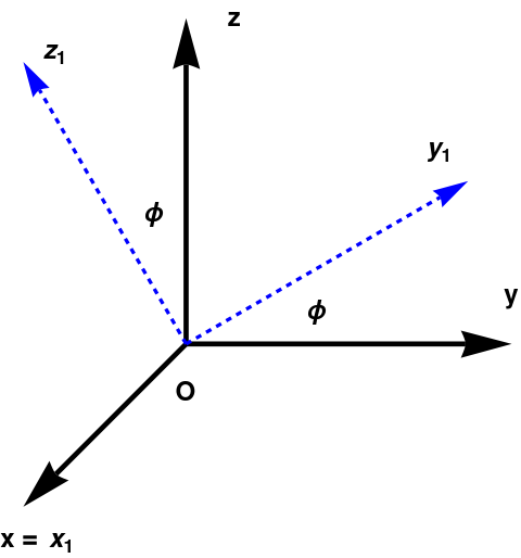
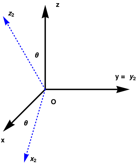
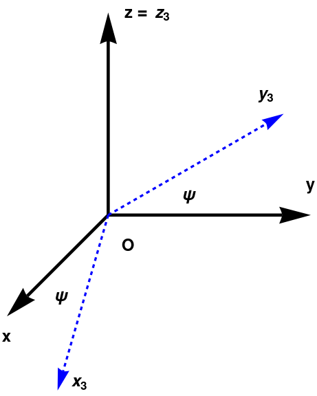
Suppose that you are a pilot, such that the x-axis points to your right, the y-axis points ahead of you, and the z-axis points up. This is the coordinate frame. Then a rotation about the x-axis, denoted by ϕ, is called the pitch. A rotation about the y-axis, denoted by θ, is called roll. A rotation about the z-axis, denoted by ψ, is called yaw. Euler’s theorem states that any position in space can be expressed by composing three such rotations, for an appropriate choice of (φ, θ, ψ (see next section).
Three dimensional orthogonal matrices have simple defining properties: each column is a unit length vector which is perpendicular to the others, and the third column is the cross product of the first two. (Rows satisfy the same properties.) The first two properties are those of orthogonality, and can be summarized as QTQ = I, the identity matrix; the last makes the orthogonality special, and can be stated as det(Q) = +1. Orthogonality alone implies that the determinant must be either +1 or –1, with the latter indicating the presence of a reflection in the matrix. A 3×3 orthogonal matrix with negative determinant can be converted to a pure rotation by factoring out a −I.
In 3D, rotation occurs about an axis rather than a point, with the term axis taking on its more common place meaning of a line about which something rotates. An axis of rotation does not necessarily have to be one of the three standard axes.
Rotation about the ordinate has a similar matrix:
The three angles ϕ, θ, ψ give a parametrization of the group of rotations, SO(3). Another parametrization will be considered in the fllowing section.
Arbitrary Axis of Rotations
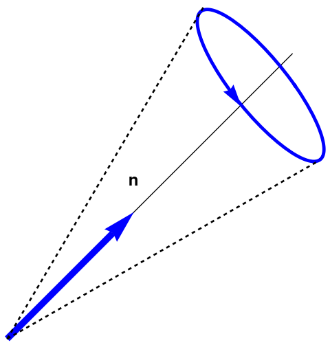
We can also rotate about an arbitrary axis in 3D, provided, of course, that the axis passes through the origin, since we are not considering general translation at the moment. This is more complicated and less common than rotating about a cardinal axis. As before, we define θ to be the amount of rotation about the axis counterclockwise. The axis will be defined by a unit vector \( \displaystyle \hat{\bf n} = ( n_x , n_y , n_z ) \) along the axis. The corresponding matrix of rotation is denoted as \( \displaystyle {\bf R} \left( \hat{\bf n}, \theta \right). \) Then the rotation of a vector v is defined by matrix multiplication:where v and u are column vectors from ℝ3×1. Be aware that in many applications a rotation matrix is used as an operator acting from left on column vectors as well as an operator acting from right on row vectors. the corresponding matrices are transposed of each other. When a matrix is multiplied from left, we write it in brackets. On the other hand, we embrace matrix in parentheses when it acts on row vectors from right.
Determination of rotation trough matrix multiplication \eqref{EqRot.4} is not computationally efficient because a rotation is specified by four parameters (angle θ and three components of axis of rotation) but 3-by-3 matrix R(n, θ) has nine entries. A more efficient algorithm is discussed in a special section on quaternions. In this section, we present two approaches for determination of rotation matrix (Mathematica has a dedicated command RotationMatrix), both based on observation that a rotation in 3D is actally a two-dimensional when plane of rotation is known.
To derive the matrix \( \displaystyle {\bf R} \left( \hat{\bf n} , \theta \right) , \) we separate v into two vectors, v∥ and v⊥, which are parallel and perpendicular to \( \displaystyle \hat{\bf n} , \) respectively, such that \( \displaystyle {\bf v} = {\bf v}_{\|} + {\bf v}_{\perp} . \) Since v∥ is parallel to n, it will not be affected by the rotation about n (namely, u∥ = v∥). So all we need to do is compute u⊥, and then we have u = v∥ + u⊥. To compute u⊥, we construct the vectors v∥, v⊥, and an intermediate vector w, as follows:
-
The vector v∥
is the portion of v that is parallel to n:
\[ {\bf v}_{\|} = \left( {\bf v} \bullet \hat{\bf n} \right) \hat{\bf n} . \]
- The vector u⊥ is the portion of v that is perpendicular to n: \( \displaystyle {\bf v} = {\bf v}_{\|} + {\bf v}_{\perp} . \)
-
The vector w is mutually perpendicular to v∥ and v⊥
and has the same length as v⊥. So
\[ {\bf w} = \hat{\bf n} \times {\bf v}_{\perp} . \]
General Observation
Two first vectors, u>₁ and u₂ must be orthogonal to u>₃ and have unit magnitudes;. Since they are arbitrary except these two properties, we can choose them wisely. So we set
The first step is to find a positive orthonormal basis of ℝ³, β = [v₁, v₂, u], where \( \displaystyle \quad {\bf u} = \left( 1/\sqrt{14} \right) \left( 2, 3, -1 \right) \quad \) is a unit vector spanning L and v₁, v₂ are an orthonormal basis for the orthogonal plane L⊥. ‘Positive’ means det[v₁|v₂|u] = 1. We start by ‘trial and error to determine one vector \( \displaystyle \quad {\bf v}_1 = \left( 1/\sqrt{5} \right) \left( 1, 0, 2 \right) \quad \) from L⊥. Another vector we determine by taking cros product \[ {\bf v}_2 = {\bf v}_1 \times {\bf u} = \frac{1}{\sqrt{70}} \left( -6, 5, 3 \right) . \]
Second step: computing the action of rotation matrix R(θ = π/6] on the basis vectors. Since u is a vector on the axis, it is fixed by R: R u = u. In the plane L⊥, R acts exactly like the counterclockwise rotation by π/6 radians in ℝ², so we know what R does to an orthonormal basis. We obtain: \begin{align*} {\bf R}\,{\bf v}_2 &= {\bf v}_2 \cos \left( \frac{\pi}{6} \right) - {\bf v}_1 \sin \left( \frac{\pi}{6} \right) = \frac{\sqrt{3}}{2}\,{\bf v}_2 - \frac{1}{2}\,{\bf v}_1 , \\ {\bf R}\,{\bf v}_1 &= {\bf v}_2 \sin \left( \frac{\pi}{6} \right) + {\bf v}_1 \cos \left( \frac{\pi}{6} \right) = \frac{1}{2}\,{\bf v}_2 + \frac{\sqrt{3}}{2}\,{\bf v}_1 , \\ {\bf R}\,{\bf u} &= {\bf u} . \end{align*} This means that the matrix of R in the ‘adapted’ basis β is: \[ [\![{\bf R}]\!]_{\beta} = \begin{bmatrix} \sqrt{3}/2 & -1/2 & 0 \\ 1/2 & \sqrt{3}/2 & 0 \\ 0&0&1 \end{bmatrix} . \] Third step. Now use the change of basis formula. We have: \[ {\bf R} = {\bf P}\,[\![{\bf R}]\!]_{\beta} {\bf P}^{-1} \] where P is the matrix of column vectors of the basis β = [v₂, v₁, u] \[ {\bf P} = \begin{bmatrix} -\frac{6}{\sqrt{70}} & \frac{1}{\sqrt{5}} & \frac{2}{\sqrt{14}} \\ \frac{5}{\sqrt{70}} & 0 & \frac{3}{\sqrt{14}} \\ \frac{3}{\sqrt{70}} & \frac{2}{\sqrt{5}} & - \frac{1}{\sqrt{14}} \end{bmatrix} . \] We check with Mathematica that such constracted matrix R is orthogonal, RTR = I, the identity matrix:

Reflections
Reflection (also called mirroring) is a transformation that “flips” the object about a line (in 2D) or a plane (in 3D). In general, it is an isometry with a hyperplane as a set of fixed points. Reflection can be accomplished by applying a scale factor of −1:In case when nomal vector a in formulas above has a unit length, we can write the reflection matrix in three-dimensional space as
Out of many linear transformations in ℝ³, only translations, rotations, uniform scale, and reflections preserve the magnitudes of angles. However, the latter may reverse the direction of the angle. The following example illustrates the general formula for reflection matrix.
Solution: The orthogonal line L is spanned by the unit vector: \[ \hat{\bf n} = \frac{1}{\sqrt{14}} \left( 2, 3, -1 \right) . \] Any vector v ∈ ℝ³ can be written as the sum of its orthogonal projections on L and on the given plane L⊥: \[ {\bf v} = \left( {\bf v} \bullet \hat{\bf n} \right) \hat{\bf n} + {\bf w} , \qquad {\bf w} = {\bf v} - \left( {\bf v} \bullet \hat{\bf n} \right) \hat{\bf n} \in L^{\perp} . \] The reflection T flips n (so Tn = −n) and fixes every w ∈ L⊥ (that is, Tw = w). By linearity of T, we have \begin{align*} T{\bf v} &= \left( {\bf v} \bullet \hat{\bf n} \right) T\hat{\bf n} + T\,{\bf w} \\ &= \left( {\bf v} \bullet \hat{\bf n} \right) \left( -\hat{\bf n} \right) + {\bf w} \\ &= - \left( {\bf v} \bullet \hat{\bf n} \right) \hat{\bf n} + \left( {\bf v} - \left( {\bf v} \bullet \hat{\bf n} \right) \right) \\ &= {\bf v} -2\left( {\bf v} \bullet \hat{\bf n} \right) \hat{\bf n} . \end{align*} Incidentally, this calculation gives a general formula for the reflection on a plane with unit normal n.) In the present case, this reads: \[ T{\bf v} = {\bf v} - \frac{2}{14}\,\left\langle {\bf v}, (2, 3, -1) \right\rangle \left( 2, 3. -1 \right) . \] In particular, \begin{align*} T\,{\bf e}_1 &= T\,{\bf i} = {\bf e}_1 - \frac{2}{7} \left( 2, 3, -1 \right) = \left( 1, 0, 0 \right) - \frac{2}{7} \left( 2, 3, -1 \right) , \\ T{\bf e}_2 &= T\,{\bf i} = {\bf e}_2 - \frac{2}{7} \left( 2, 3, -1 \right) = \left( 0, 1, 0 \right) - \frac{2}{7} \left( 2, 3, -1 \right) , \ T{\bf e}_3 &= T\,{\bf i} = {\bf e}_3 - \frac{2}{7} \left( 2, 3, -1 \right) = \left( 0, 0, 1 \right) - \frac{2}{7} \left( 2, 3, -1 \right) . \end{align*} These vectors form the matrix T in standard basis: \[ {\![ T]\!] = \frac{1}{7} \begin{bmatrix} 3 & -4& -4 \\ -6 &1 & -6 \\ 2 & 2& 9 \end{bmatrix} . \]
-
Verify directly that the following 3 × 3 matrices define rotation transformation along the line through the origin and the point (1, 1, 1).
- A rotation by π/6 (= 30°) is \( \displaystyle \quad \frac{1}{3} \begin{bmatrix} \left( 1 + \sqrt{3} \right) & 1 & \left( 1 - \sqrt{3} \right) \\ \left( 1 - \sqrt{3} \right) & \left( 1 + \sqrt{3} \right) & 1 \\ 1 & \left( 1 - \sqrt{3} \right) & \left( 1 + \sqrt{3} \right) \end{bmatrix} ; \)
- A rotation by π/3 (= 60°) is \( \displaystyle \quad \frac{1}{3} \begin{bmatrix} 2&2&-1 \\ -1&2&2 \\ 2&-1&2 \end{bmatrix} ; \)
- A rotation by π/2 (= 90°) is \( \displaystyle \quad \frac{1}{3} \begin{bmatrix} 1& \left( 1 + \sqrt{3} \right) & \left( 1 - \sqrt{3} \right) \\ \left( 1 - \sqrt{3} \right) & 1 & \left( 1 + \sqrt{3} \right) \\ \left( 1 + \sqrt{3} \right) & \left( 1 - \sqrt{3} \right) & 1 \end{bmatrix} ; \)
- A rotation by 2π/3 (= 120°) is \( \displaystyle \quad \begin{bmatrix} 0&1&0 \\ 0&0&1 \\ 1&0&0 \end{bmatrix} . \)
- For a given angle θ, you can write six matrices that define rotations along coordinate vectors i, −i, j, −j, k, and −k. Their inverse matrices give six more matrix expressions. Another twelve expressions are formed by putting −θ for θ. Break these twenty four matrix expressions into a separate lists so that the expressions in each list are necessarily equal but any two matrices from different lists are not equal in general. For example, R(i, θ) and (R(−j, θ))−1 are equal and so are in the same list.
- Find all 3 × 3 rotation matrices that are also diagonal.
- Show that a nonzero 3 × 3 matrix P is a rotation if and only if the rows of P have the same cross-product relation as i, j, k; for example, 1row × 2row = 3roe.
- Anton, Howard (2005), Elementary Linear Algebra (Applications Version) (9th ed.), Wiley International
- Coxeter, H.S.M. (1969), Introduction to Geometry (2nd ed.), New York: John Wiley & Sons, ISBN 978-0-471-50458-0
- Dunn, F. and Parberry, I. (2002). 3D math primer for graphics and game development. Plano, Tex.: Wordware Pub.
- Foley, James D.; van Dam, Andries; Feiner, Steven K.; Hughes, John F. (1991), Computer Graphics: Principles and Practice (2nd ed.), Reading: Addison-Wesley, ISBN 0-201-12110-7
- Matrices and Linear Transformations
- Rogers, D.F., Adams, J. A., Mathematical Elements for Computer Graphics, McGraw-Hill Science/Engineering/Math, 1989.
- Watt, A., 3D Computer Graphics, Addison-Wesley; 3rd edition, 1999.