Suppose that V is finite-dimensional vector space and let β = { e1, e2, … , en }
be a basis of V. For each i = 1, 2, … , n, define a linear functional ej : V ↦ 𝔽 by setting
It is customary to denote dual bases in V ′ (V✶) by the same letters as corresponding bases in V but using lower indices ("downstairs") for V and upper indices ("upstairs") for V ′ (V✶). Then every vector v = viei in V has coordinates vi with upper indeces, so the dual vector φ = φiei in V ′ (V✶) is uniquely identified by objects φi with lower indeces. It is convenient to use the Einstein summation convention and drop the summation symbol ∑. In this language, the canonical isomorphism between V and V ′ (V✶) is realized by
lowering and raising indices. The upper index object vi represents the coordinate vector relative to a basis ei of V and is also called the contravariant vector.
The lower index object φi is the i-th coordinate of dual vector relative to the dual basis ei and is also called covariant vector.
Theorem 2:
The set β* is a basis of V ′. Hence, V ′ is finite-dimensional and dim(V ′) = dim(V).
First we check that the functionals { e1, e2, … , en } are linearly independent. Suppose that there exist 𝔽-scalars k1, k2, … , kn so that
Note that the 0 on the right denotes the zero functional; i.e., the functional that sends
everything in V to 0 ∈ 𝔽. The equality above is an equality of maps, which should hold
for any v ∈ V we evaluate either side on. In particular, evaluating both sides on every element from the basis β, we have
Again, this means that both sides should give the same result when evaluating on any v ∈ V. By linearity, it suffices to check that this is true on the basis β. Indeed, for each i, we get
again by the definition of the ei and the bi. Thus, φ and b1e1 + ⋯ + bnen agree on the basis, so
we conclude that they are equal as elements of V*. Hence {e1, e2, … , en} spans V* and therefore
forms a basis of V*.
Example 5:
In vector space ℝ³, let us consider a (not orthogonal) basis
Now suppose that we realize that I made a typo enterning matrices e₁, e₂, e₃. Suppose that in entries of vector e₃ I made one mistake and base vectors must be as follows:
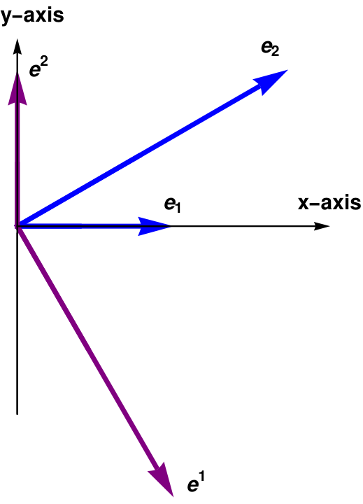
Flat space ℝ²: We consider the simplest example that allows us to visualize the basis vectors and corresponding dual vectors.
The basis vectors need be neither normalized (having unit length) nor orthogonal, it doesn’t matter. In this case,
the basis vectors [e₁, e₂] are not simulteneously normalized for simplicity. Given the ordered basis set [e₁, e₂] for vector space ℝ², a corresponding
basis set of dual vectors [e¹, e²] is defined by:
As shown on Figure 5.1, the dual basis vectors are perpendicular to all basis vectors
with a different index, and the scalar product of the dual basis vector with the basis vector of the
same index is unity. The basis set for dual vectors enables any dual vector φ to be written:
\[
\varphi = \varphi_1 \mathbf{e}^1 + \varphi_2 \mathbf{e}^2 = \varphi_{\alpha} \mathbf{e}^{\alpha} ,
\]
where coefficients are not determined by perpendicular projections onto
the basis vector as for Cartesian components but by tracing a parallelogram.
Already the usefulness of the Einstein summ
The usefulness of the Einstein summation rule is apparent: Any term containing a dummy
variable forces a summation, in this case only over α = 1, 2.
The set of basis vectors (in blue) and their corresponding covectors (in purple) for the example in Figure 5.1 are
\begin{align*}
\mathbf{e}_1 &= \left( 1, 0 \right) , \qquad \mathbf{e}_2 = \left( \sqrt{3}, 1 \right) ;
\\
\mathbf{e}^1 &= \left( 1 , - \sqrt{3} \right) , \qquad \mathbf{e}^2 = \left( 0, 1 \right) ,
\end{align*}
which satisfy Eq. (1).
■
End of Example 5
There does exist a unique correspondence between ordered basis sets in V
and its dual V ′ (V✶)
but not between individual vectors in V
and its dual V ′ (V✶). Moreover, changing only one element of a basis β in V changes several elements in the dual basis β* (see Example 5).
Corollary 1:
Let φ ∈ V ′ (V✶) be a nonzero functional on V, and let v ∈ V be any element such that φ(v) = <φ|v> ≠ 0.Then V is a direct sum of two subspaces:
Let v ∈ V be a vector that is not annihilated by linear form φ(v) = <φ|v> ≠ 0. Then we can choose a basis β of V such that β = { e1 = v, e2, … , en }, so that the first vector in this set is v. Let β* = { e1, e2, … , en } be a dual basis in V*. By definition of dual basis, e1(v) = 1, and for all other basis elements, we have
e1(ej) = 0, j = 2, 3, … , n. We can prove that kerφ⊂span{e2, … , en} and span{e2, … , en}⊂kerφ, so kerφ=span{e2, … , en}.
Therefore, the kernel (or null space) of e1 is n − 1 dimensional.
Hence, the functional φ has the following representation in the dual basis:
\[
\phi = \phi ({\bf v})\,{\bf e}^1 = c\, {\bf e}^1 , \qquad c\ne 0.
\]
This functional maps the rest basis elements { e2, … , en } to zero, so V = span(v) ⊕ kerφ because every vector u ∈ V has a unique representation
\[
{\bf u} = c^1 \cdot {\bf e}_1 + c^2 \cdot {\bf e}_2 + \cdots + c^n \cdot{\bf e}_n ,
\]
and
\[
{\bf v} = {\bf e}_1 = {\bf e}_1 + 0\cdot {\bf e}_2 + \cdots + 0\cdot{\bf e}_n .
\]
Example 6:
We identify the two dimensional vector space ℂ² of ordered pairs (z₁, z₂) of two complex numbers with its isomorphic image of column vectors:
We consider a linear form
\[
\varphi \left( z_1 , z_2 \right) = z_1 - 2{\bf j}\, z_2 .
\tag{6.1}
\]
As usual, j denotes a unit imaginary vector in ℂ, so j² = −1.
The kernel of φ consists of all pairs of complex numbers (z₁, z₂) for which z₁ = 2jz₂. Hence, the null space of φ is spanned on the vector
\[
\mbox{ker}\varphi = \left\{ \left[ \begin{array}{c} 2{\bf j}\,y \\ y \end{array} \right] : \quad y \in \mathbb{C} \right\} .
\tag{6.2}
\]
Let z = (z₁, z₂) be an arbitrary vector from ℂ²,and v = (1+j, 1−j) be given. We have to show that there is a unique decomposition:
\[
{\bf z} = \left( z_1 , z_2 \right) = c\left( 1 + {\bf j}, 1 - {\bf j} \right) + \left( 2{\bf j}, 1 \right) y ,
\tag{6.3}
\]
where y∈ℂ is some complex number. Equating two components, we obtain two complex equations:
\[
\begin{split}
z_1 &= c \left( 1 + {\bf j} \right) + 2{\bf j}\, y ,
\\
z_2 &= c \left( 1 - {\bf j} \right) + y .
\end{split}
\tag{6.4}
\]
Since the matrix of system (6.4) is not singular,
\[
{\bf A} = \begin{bmatrix} 1 + {\bf j} & 2{\bf j} \\ 1 - {\bf j} & 1 \end{bmatrix} \qquad \Longrightarrow \qquad \det{\bf A} = -1-{\bf j} \ne 0 ,
\]
1 + I - 2*I*(1 - I)
-1 - I
system (6.4) has a unique solution for any input z = (z₁, z₂):
\[
c = \frac{1 + {\bf j}}{2} \left( z_1 - 2{\bf j}\, z_2 \right) , \qquad y = - z_2 - {\bf j}\, z_1 .
\]
{{c -> (-(1/2) + I/2) (z1 - 2 I z2), y -> -I (z1 - I z2)}}
■
End of Example 6
In other words, any vector v not in the kernel of a linear functional generates a supplement of this kernel: The kernel of a nonzero linear functional has codimension 1. When V is finite dimensional, the rank-nullity theorem claims:
If a vector space V is not trivial, so V ≠ {0}, then its dual V* ≠ {0}.
Theorem 3:
Let φ, ψ be linear functionals on a vector space V. If φ vanishes on ker(ψ), then φ = cψ is a constant multiple of ψ.
If ψ = 0, there is nothing to prove. Let us assume that ψ ≠ 0, and
choose a vector x ∈ V such that ψ(x) ≠ 0. Consider the linear functional ψ(x)φ − φ(x)ψ,
which vanishes on x and on kerψ by assumption. By Corollary 1, this linear functional vanishes identically: We get a linear dependence relation.
Another proof:
∀ ϕ ∈ V*, ∃ x such that ϕ(x) ≠ 0, according to Corollary 1, V = span(x) ⊕ kerϕ ⇒ ∀ v ∈ V, v = cx + y, y ∈ kerϕ ⇒ ψ(v) = ψ(cx + y) = ψ(cx) + ψ(y) = cψ(x) + 0 = c ψ(x)/ϕ(x) ϕ(x) + ϕ(y) = ψ(x)/ϕ(x) ϕ(cx) +ψ(x)/ϕ(x) ϕ(y) = ψ(x)/ϕ(x) ϕ(cx + y) = ψ(x)/ϕ(x ) ϕ(v).
Example 7:
We consider V = ℝ3,3, the set of all real-valued 3×3 matrices, and φ a linear functional on it:
where tr(M) is the trace of matrix M. The dimension of V is 9. Functional φ annihilates matrix M if and only if its trace is zero:
\[
a_{11} + a_{22} + a_{33} = 0 ,
\]
which imposes one condition (linear equation) on the coefficients of matrix M. Therefore, the kernel (null space) of φ is 8-dimensional (9 − 1 = 8). The image of φ is just ℝ, that is, one-dimensional vector space.
Trace is the sum of the diagonal elements in a matrix. Here is how Mathematica computes the Trace.
Theorem 4:
Let φi ∈ V* (1 ≤ i ≤ m)
be a finite set of linear functionals. If a linear functional ψ ∈ V* vanishes on intersection \( \displaystyle \cap_{1 \leqslant i \leqslant m} \mbox{ker}\varphi_i , \) then ψ
is a linear combination of the φi, so ψ ∈ span(φ1, … , φm).
Let us proceed by induction on m. For m = 1, it is the
statement of Theorem 3. Let now m ≥ 2, and consider the subspace
\[
W = \cap_{1 \leqslant i \leqslant m} \mbox{ker}\varphi_i \supset W \cap \mbox{ker}\varphi_1 ,
\]
as well as the restrictions of ψ and φ1 to W. By assumption, \( \displaystyle \left. \psi\right\vert_{W} \) vanishes on
kerφ1|W. Hence there is a scalar c such that
ψ|V = cφ1|V, namely,
ψ − cφ1 vanishes on W. By the induction assumption, ψ − cφ1 is a linear combination of φ2, … , φm, say
Another way to prove this theorem is to to construct a basis according to the following algorithm.
Let β = { }.
Choose φj from the given finite set of linear functionals.
If φj vanishes on the kernel of any linear functional in β, do nothing and start from 2 again. Else, ∃vj∈V, such that φj(vj)≠0, and we can scale vj to make φj(vj)=1. We then add vj to β.
Let's suppose that after going through the given finite set of linear functionals, we have β = {v1, … , vr}, then either β is a basis for the vector space V, or we can expand it to a basis for the vector space V, such as β = {v1, … , vr, ur+1, … , un}, and there is φj in our given finite set of linear functionals such that φj(vj) = 1. Further more, it is not hard to prove that ∩1≤j≤mker(φj) = span(ur+1, … , un).
For such basis β of the vector space V, there is corresponding basis β* = {e1, … , er, er+1, … , en} of dual space V*, in which ej = φj. For any φ ∈ V*, \( \displaystyle \varphi = \sum_{i=1}^n c_i {\bf e}^i . \) Since φ vanishes on ∩1≤j≤mker(φj), cj = 0 for j = r+1, … , n. Then we have
\[
\varphi = \sum_{j=1}^n c_j {\bf e}^j =\sum_{j=1}^r c_j {\bf e}^j = \sum_{j=1}^r c_j \varphi_j .
\]
Example 8:
Let ℝ≤n[x] be a set of polynomials in variable x of degree up to n with real coefficients. As we know, the monomials ek(x) = xk (k = 0, 1, 2, … , n) form a standard basis in this space.
where \( \displaystyle n^{\underline{j}} = n \left( n-1 \right) \left( n-2 \right) \cdots \left( n-j+1 \right) \) is the j-th falling factorial. As usual, we denote by \( \displaystyle \texttt{D}^0 = \texttt{I} \) the identity operator, and 0! = 1. It is not hard to check that ej form a dual basis for monomials xi. Indeed, substituting p(x) = xk into Eq.(8.1), we get
So we need to check the case j = k. In this case, the falling factorial becomes the regular factorial, \( \displaystyle k^{\underline{k}} = k! , \) , so
This polynomial expansion is well-known in Calculus as the Maclaurin formula.
(The Maclaurin formula is represented as a form of Taylor Series in Mathematica.)
Let us consider the linear form
\[
\psi \left( p(x) \right) = p(0) + p' (0) .
\]
This functional vanishes on the intersection of kernels ker(e0) ∩ ker(e1) ⊂ker(ψ). Therefore, ψ = c₀e0 + c<₁b>e1, for some scalars c₀ and c₁.
■
End of Example 8
Since a vector space V and its dual V ′ (V✶) have the same dimension, hence, they are isomorphic. In general, this isomorphism depends on a choice of bases. However, a canonical isomorphism (known as Riesz representation theorem) between V and its dual V* can be defined if V carries a
non-degenerate inner product.
Theorem 5:
If v and u are any two distinct vectors of the n-dimensional vector space V, then there exists a linear functional φ on V such that <φ|v> ≠ <φ|u>; or equivalently, to any nonzero vector v ∈ V, there corresponds a ψ ∈ V* such that
<ψ|v> ≠ 0.
This theorem contains two equivalent statements because we can always consider the difference u − v to reduce the first statement to the homogeneous case. So we prove only the latter.
Let β = { e1, e2, … , en } be any basis in vector space V, and let β* = { e1, e2, … , en } be the dual basis in V*. If
\( {\bf v} = \sum_i k_i {\bf e}_i , \) then <ej|v> = ki. Hence, if <ψ|v> = 0 for all ψ, in particular, if <ej|v> = 0 for all j = 1, 2, … , n, then v = 0.
Example 9:
Let V = ℭ[0, 1] be the set of all continuous functions on the interval [0, 1]. Let f and g be two distinct continuous functions on the interval. Then there exists a point 𝑎 ∈ [0, 1] such that f(𝑎) ≠ g(𝑎). Let us consider a linear functional δ𝑎 that maps these two functions f and g into different real values. Indeed, let
\[
\delta_a (f) = f(a) .
\]
Then δ𝑎 is a required functional that distinguishes f and g. As it is widely used in applications, the functional above can be written with the aid of the Dirac delta function:
\[
\int_0^1 \delta (x-a)\,f(x)\,{\text d} x = f(a) .
\]
■
End of Example 9
From Theorem 5, it follows that a functional on any finite-dimensional vector space is unique; this means that if φ(v) = 0 for every v ∈ V, then φ ≡ 0.
Theorem 6:
Let V be an n-dimensional space with a basis β = { e1, e2, … , en }. If { k1, k2, … , kn } is any list of n scalars, then there is one and only one linear functional φ on V such that φ(ei) = < φ | ei > = ki for i = 1, 2, … , n.
For the existence statement, we can just construct this linear transformation:
\[
\varphi ({\bf e}_i ) = \langle \varphi \mid {\bf e}_i \rangle = k_i , \qquad i=1,2,\ldots , n ,
\]
where β = {e1, e2, … , en} is a basis in V.
Every v in V can be written in the form v = s1e1 + s2e2 + ⋯ + snen in one and only one way because β is a basis. If ψ is any linear functional, then
then ψ is indeed a linear functional and <ψ|ei> = ki.
Example 10:
Let 𝑎1, 𝑎2, … , 𝑎n+1 be distinct points (in
ℝ or ℂ), and let ℝ≤n[x] be the space of polynomials of degree at most n in variable x. Define
n+1 linearly independent functionals
where j in the products runs from 1 to n + 1. The set of Lagrange polynomials β = {p1(x), p2(x), … , pn+1(x)} is a basis in the space ℝ≤n[x]. First, they all are polynomials of degree n, so (10.1) are elements of the vector space ℝ≤n[x]. Second, the Lagrange polynomials are linearly independent. Indeed, suppose that their linear combination is identically zero (for any x)
\[
b_1 p_1 (x) + b_2 p_2 (x) + \cdots + b_{n+1} p_{n+1} (x) = 0 ,
\tag{10.2}
\]
with some scalars b1, b2, … , bn+1 ∈ ℝ. The relation (10.2) must hold for any x because it must be valid in sense of functions (two functions f and g are equal if and only if f(x) = x(g) for any entry x from the domain---ℝ in our case). We evaluate the relation (10.2) at every point 𝑎j and get
\[
b_1 p_1 (a_j ) + b_2 p_2 (a_j ) + \cdots + b_{n+1} p_{n+1} (a_j) = b_j = 0 , \qquad j=1,2,\ldots , n+1 .
\tag{10.3}
\]
Since the numerator of polynomial pk(x) is a product of n simple monomials (x − 𝑎j) that vanish at x = 𝑎j, we have pk(𝑎k) = 1 and
pk(𝑎j) = 0 if j ≠ k, so every coefficient bj in Eq.(10.2) is zero. This proves that the set of Lagrange polynomials is linearly independent. Since there are exactly n + 1 distinct polynomials, we claim that the Lagrange polynomials (10.1) constitute a basis in the space ℝ≤n[x].
Hence,
the system p1(x), p2(x) , … , pn+1(x) is dual to the system φ1, φ2, … , φn+1 in the sense that ⟨φk∣pj⟩ = δk,j the Kronecker delta.
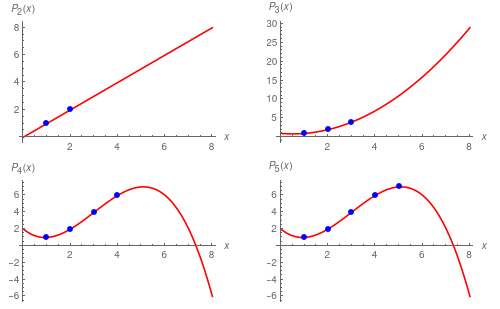
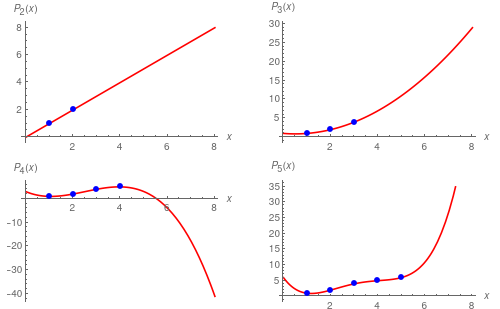
Now we can construct a polynomial that makes specified values at the given list of points 𝑎1, 𝑎2, … , 𝑎n+1:
Note in the output below, each graphic has a different label for each y axis as the k in Subscript[p, k] increments higher; and the number of points coincide with the value of the k subscript. Accordingly, the product of these approaches the true functional form with added increments.
Lagrange intepolation polynimials P₂, P₃, P₄, and P₅.
Note a small difference in the choice of points makes a considerable difference in the shape of the function.
Theorem 7:
Let β = [e₁, e₂, … , en] be an ordered basis of a finite-dimensional vector space V over a field 𝔽, and let ψ : V ⇾ 𝔽 be a linear functional. Then there exists a unique vector v ∈ V such that
\[
\psi (\mathbf{u}) = [\![ \mathbf{v}]\!]_{\beta} \bullet [\![\mathbf{u}]\!]_{\beta} ,
\]
where ⟦v⟧β = [v₁, v₂, … , vn] and ⟦u⟧β = [u₁, u₂, … , un] are coordinate vector representations of v = v₁e₁ + v₂e₂ + ⋯ + vnen and u = u₁e₁ + u₂e₂ + ⋯ + unen with respect to basis β, respectively.
Since ψ is a linear transformation, Theorem 6 of section tells us that it has a
standard matrix—a matrix A such that ψ(u) = A ⟧u⟦β for all u ∈ V. Since ψ maps into 𝔽, which is 1-dimensional, the standard matrix A is 1 × n, where n = dim(V). It follows that A is a row vector, and since every vector in 𝔽n ≌ 𝔽1×n is the coordinate vector of some vector in V, we can find some v ∈ V such that A = ⟧v⟦β, so that ψ(u) = ⟧v⟦β • ⟧u⟦β.
Uniqueness of vector v follows immediately from uniqueness of standard matrices and of coordinate vectors.
Example 11:
We consider a linear functional on the set of polynomials of degree no more than 3, inclusive P≤3⟦x⟧:
\[
\psi_r (p) = p(r), \qquad p(x) = a + b\, x + c\, x^2 + d\, x^3 \in P_{\le 3}[\![x]\!] .
\]
Let β = [1, x, x², x³] be a standard basis in P≤3⟧x⟦. Then every polynomial can be written as p(x) = 𝑎 + b x + c x² + d x³, then ⟧p(x)⟦β = [𝑎, b, c, d]. Applying the functional ψ, we get
\[
\psi_r (p) = a + b\,r + c\,r^2 + d\,r^3 = \left( 1, r, r^2 , r^3 \right) \bullet \left( a, b, c, d \right) .
\]
■