
Introduction to Linear Algebra
Systems of Linear Equations
- Introduction
- Linear systems
- Vectors
- Linear combinations
- Matrices
- Planes in ℝ³
- Reduced Row-Echelon Form
- Equation A x = b
- Sensitivity of solutions
- Linear independence
- Plane transformations
- Space transformations
- Linear transformations
- Affine maps
- Exercises
- Answers
Matrix Algebra
- Introduction
- Manipulation of matrices
- Partitioned matrices
- Block matrices
- Matrix operators
- Determinants
- Cofactors
- Cramer's rule
- Equivalent matrices
- Elimination: A = L U
- PLU factorization
- Reflection
- Givens rotation
- Special matrices
- Exercises
- Answers
Vector Spaces
- Introduction
- Motivation
- Vector spaces
- Bases
- Dimension
- Coordinate systems
- Linear transformations
- Change of basis
- Matrix transformations
- Compositions
- Isomorphisms
- Dual transformations
- Quotient spaces
- Wedge products
- Rotors
Eigenvalues, Eigenvectors
- Introduction
- Characteristic polynomials
- Companion matrix
- Algebraic and geometric multiplicities
- Minimal polynomials
- Eigenspaces
- Where are eigenvalues?
- Eigenvalues of A B and B A
- Generalized eigenvectors
- Similarity
- Diagonalizability
- Self-adjoint operators
- Exercises
- Answers
Euclidean Spaces
- Introduction
- Euclidean space
- Bilinear transformations
- Norm and distance
- Matrix norms
- Dual norms
- Dual transformations
- Examples of transformations
- Orthogonality
- Gram--Schmidt Process
- Orthogonal matrices
- Self-adjoint matrices
- Unitary matrices
- Projection operators
- QR-decomposition
- Least Square Approximation
- Quadratic forms
- Exercises
- Answers
Canonical forms
- Introduction
- 2D decomposition
- 3D decomposition
- Projectors
- Direct-sum decompositions
- Cyclic decompositions
- Symmetric matrices
- Symmetric matrices
- Pseudoinverse
- URV-decomposition
- LU-decomposition
- QR-decomposition
- Cholesky decomposition
- Schur decomposition
- Positive matrices
- Roots
- Polar factorization
- Spectral decomposition
- CUR decomposition
- Exercises
- Answers
Applications
- Introduction
- Circles along curves
- TNB frames
- GPS problem
- Poisson equation
- Graph theory
- Error correcting codes
- Electric circuits
- FSA
- Markov chains
- Cryptography
- Wave-length transfer matrix
- Computer graphics
- Linear Programming
- Hill's determinant
- Fibonacci matrices
- Discrete dynamic systems
- Discrete Fourier transform
- Fast Fourier transform
- Curve fitting
- Answers
Miscellany
- Introduction
- Circles along curves
- TNB frames
- Differential forms
- Calculus
- Vector representations
- Matrix representations
- Change of basis
- Orthonormal Diagonalization
- Generalized inverse
- Differential forms
Preliminaries
- Complex Number Operations
- Sets
- Polynomials
- Polynomials and Matrices
- Computer solves Systems of Linear Equations
- Location of Eigenvalues
- Power Method
- Iterative Method
- Similarity and Diagonalization
Glossary
Reference

This Book is licensed under Creative Commons Attribution-NonCommercial-NoDerivs 3.0 Unported License
This section is divided into a number of subsections, links to which are:
Python:
http://www.kostasalexis.com/frame-rotations-and-representations.html
https://github.com/joycesudi/quaternion/blob/main/quaternion.py
Euler Rotation Theorem
A two-dimensional x-y coordinate frame can be considered to be a part of the three-dimensional coordinate frame by adding a z-axis perpendicular to the x- and y-axes. However, there are two orientations for this line: one in which the positive direction of the axis is out of the paper and another where the positive direction of the axis is into the paper. It doesn’t matter which one we choose as long as the choice is consistent.
Consistency is made more difficult when the sciences do not agree. Elsewhere we have made a point about how physicists and mathematicians do not agree on a notation for the imaginary unit in the complex plane ℂ. Similarly, and confusingly, geometers and topologists cannot agree on a convention for numbering coordinates in space underlying equations. A useful article covering this may be found in the Hypersphere section of Wolfram MathWorld at this link. The message here is that you must adapt your consistency to the context and conform to parochial rules laid down by those who passed before you.
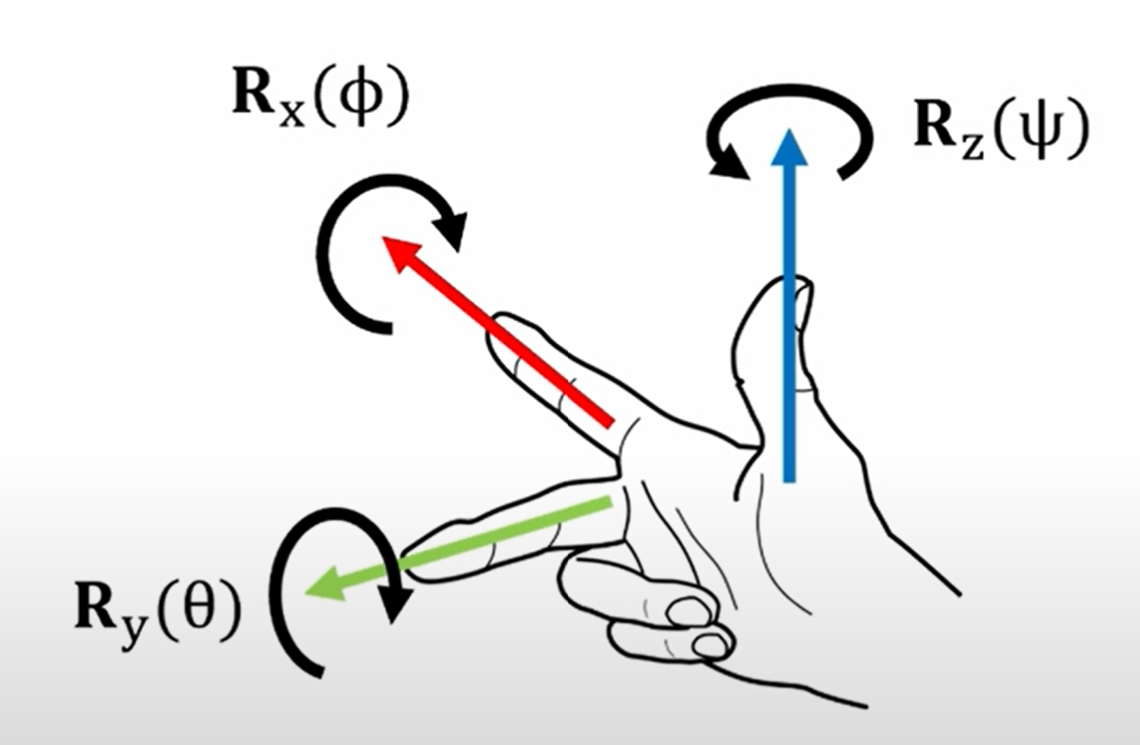
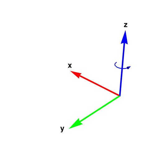
The conventional choice for labeling (orientation) axes is the right hand rule. Curl the fingers of your right hand so that they go by the shortest path from the one axis to another axis. Your thumb now points in the positive direction of the third axis. For the familiar x- and y-axes on paper, curl your fingers on the short 90° path from the x-axis to the y-axis (not on the long 270° path from the x-axis to the y-axis). When you do so your thumb points out of the paper and this is taken as the positive direction of the z-axis.
The following diagram shows the right-hand coordinate system. Note that the arrow is a semi-circle that begins and ends touching the y plane. The arrow direction is the same as the curl of your fingers.
- x-axis (abscissa) forward the index finger;
- y-axis (ordinate)up from the middle finger;
- z-axis up, from the thumb (applicate).
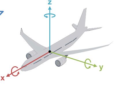
- Roll ϕ about x-axis;
- Pitch θ about y-axis;
- Yaw ψ about z-axis.
|
|

|
|
|
Leonhard Euler proved the following theorem in 1775 that states that in three-dimensional space, any displacement of a rigid body such that a point on the rigid body remains fixed, is equivalent to a single rotation about some axis that runs through the fixed point.
- Anderson, R.U., Elementary geometric proof of Euler's rotation theorem, 2019.
The parameterization of rotation through Euler angles is probably the most commonly employed in both education and engineering applications. There are three axes in three dimensional space, so there should be 3³ = 27 sequences of Euler angles. However, there is no point in rotating around the same axis twice in succession because the same result can be obtained by rotating once by the sum of the angles, so there are only 3 · 2 · 2 = 12 different Euler angle sequences:
| xyx | xyz | xzx | xzy | |||
| yxy | yxz | yzx | yzy | |||
| zxy | zxz | zyx | zyz |
We refer to this class of 12 sequences of three partial rotations as Eulerian angle parametrizations. As you see, there is no constraint to use the same axis twice interrupted by rotation with respect to another axis. Euler angles express a rotation as a sequence of three standard rotations about a predefined set of coordinate axes, in a predefined order. These standard rotations are either by convention extrinsic about the fixed global x, y, and z-axes, or intrinsic about the local x, y, and z-axes of the coordinate frame being rotated. For each of these two types, the order of axis rotations leads to six possible conventions where the first and third axes of rotation are the same, referred to as proper Euler angles:
| xyx | xzx | yxy | yzy | zxz | zyz |
Another six possible conventions where each axis is used only once, referred to as Tait-Bryan angles:
| XYZ | XZY | YXZ | YZX | ZXY | ZYX |
Classic Euler's angles usually take the inclination angle in such a way that zero degrees represent the vertical orientation. Alternative forms were later introduced by a Scottish mathematical physicist Peter Guthrie Tait (1831--1901) and an English applied mathematician George H. Bryan (1864--1928) intended for use in aeronautics and engineering in which zero degrees represent the horizontal position.
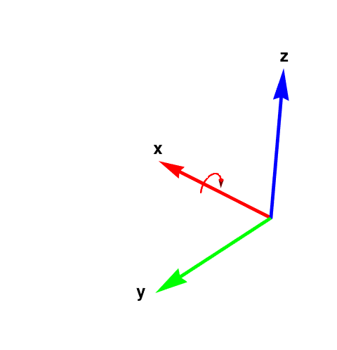
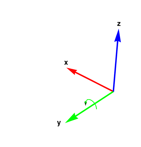
The representation is unique, except at gimbal lock, which is when θ = ± π/2 . The rotation matrix R corresponding to the Euler angles rotation E = (ψ, θ, φ) is given by \begin{align*} {\bf R} &= {\bf R}_z (\psi )\,{\bf R}_y (\theta ) \, {\bf R}_x (\phi ) \\ &= \end{align*} For example, let us start rotation with respect to vertical z-axis.
To be checked ????
Example 1 allowed rotations of a vector around the axes zyx by 90° each. The matrix for arbitrary rotations around these axes is obtained by multiplying the matrices for each axis using arbitrary angles: a rotation of ψ around the z-axis, a rotation of θ around the y-axis and a rotation of φ around the x-axis. The resulting matrix is computed as follows. First multiply the rotation around the x-axis by the rotation around the y-axis:Unfortunately, there are dozens of mutually exclusive ways to define Euler angles. Different authors are likely to use different conventions, often without clearly stating the underlying assumptions, which makes it difficult to combine equations and code from more than one source. In this tutorial, we mostly use classical Yaw-pitch-roll rotation order, rotating around the z, y and x axes respectively. There are some others:
- The three elemental rotations may be extrinsic (rotations about the axes xyz of the original coordinate system, which is assumed to remain motionless), or intrinsic (rotations about the axes of the rotating coordinate system XYZ, solidary with the moving body, which changes its orientation with respect to the extrinsic rotation. So in intrinsic system axes move with each rotation. In an extrinsic system, each rotation is performed around the axes of the world coordinate system, which does not move. As an example, suppose the three angles of the Euler triplet specify rotations around the z, y, and x axes respectively, and in that order. The first elemental rotation around the z axis will be identical for both intrinsic and extrinsic conventions. However, for the intrinsic convention the second elemental rotation is performed around the y axis in its new position resulting from the first rotation, while in the extrinsic convention it is performed around the original (unrotated) y axis. Similarly, the final rotation around the x axis will be performed around the x axis as rotated by the first two operations in the intrinsic system, and around the original (unrotated) x axis in the extrinsic system. It can be shown that all extrinsic Euler's angles conventions are completely equivalent to the corresponding intrinsic Euler's angles conventions, just with the order of rotations reversed. In this section we will adhere to the intrinsic convention: i.e., the axes move with each rotation.
- Active (otherwise known as alibi) rotation when the point is rotated, not the coordinate system.
- Passive rotation—also known as alias rotation—is when the coordinate system rotates with respect to the point . The two conventions produce opposite rotations.
- Right-handed coordinate system with right-handed rotations. We will use a right-handed Cartesian coordinate system with right-handed rotations. In a right-handed coordinate system, if x̂, ŷ, and ẑ̂ are unit vectors along each of the three axis, then x̂ cross ŷ = ẑ. Right-handed rotation means rotations are positive clockwise when looking in the positive direction of any of the three axes.
The matrix for an arbitrary rotation
The order in which the rotations are performed is significant. The primary problem with Euler angles is that they contain singularities at 0 or 90 degrees that lead to gimbal lock. When this occurs, 2 axes are parallel and it is not possible to rotate independently about a third “locked” axis. For example, if using Euler angles to describe an airplane that is rotated upward 90 degrees about it’s pitch axis so that it is pointing straight up, the yaw and roll axes become the same, and one degree of freedom is lost or “locked”. In this case, it’s not possible to independently describe tilt towards the left or right wings.
https://www.sagemotion.com/blog/how-do-euler-angles-work https://danceswithcode.net/engineeringnotes/rotations_in_3d/rotations_in_3d_part1.html
|
|
If the application of Euler angles doesn’t involve angles at or near the singularities, then this problem goes away (e.g., commercial airplanes don’t fly vertically). Euler angles can also be computed by converting from 3D rotation matrix:
Euler--Rodrigues' rotation formula
If v is a vector in ℝ³ and n is a unit vector describing an axis of rotation about which v rotates by an angle θ according to the right hand rule, the Euler--Rodrigues formula for the rotated vector vrot is
The rotation matrix can be expressed through the cross-product matrix:
For derivation of the exponential formula \eqref{EqEuler.3}, we need the characteristic polynomial of matrix K:
Under the rotation, the component v∥ parallel to the axis will not change magnitude nor direction: \( \displaystyle \quad {\bf v}_{\parallel\,rot} = {\bf v}_{\parallel} ; \quad \) while the perpendicular component will retain its magnitude but rotate its direction in the perpendicular plane spanned by v⊥ and n × v, according to \[ {\bf v}_{\perp\,rot} = {\bf v}_{\perp} \cos\theta + \left( \hat{\bf n} \times {\bf v} \right) \sin\theta = {\bf v}\, \cos\theta + \left( \hat{\bf n} \times {\bf v} \right) \sin\theta , \] in analogy with the planar polar coordinates (r, θ) in the Cartesian basis ex = i, ey = j: \[ {\bf r} = r\,\cos\theta \,{\bf e}_x + r\,\sin\theta\, {\bf e}_y = r\,\cos\theta \,{\bf i} + r\,\sin\theta\, {\bf j} . \] Now the full rotated vector is: \[ {\bf r}_{rot} = {\bf v}_{\parallel\,rot} + {\bf v}_{\perp\,rot} = {\bf v}_{\parallel} + {\bf v}_{\perp} \cos\theta + \left( \hat{\bf n} \times {\bf v} \right) \sin\theta . \] substituting \( \displaystyle \quad {\bf v}_{\perp} = {\bf v} - {\bf v}_{\parallel} \quad\mbox{or} \quad {\bf v}_{\parallel} = {\bf v} - {\bf v}_{\perp} \quad \) in the last expression gives respectively: \begin{align*} {\bf v}_{rot} &= {\bf v}\,\cos\theta + \left( 1 - \cos\theta \right) \left( \bullet {\bf v} \right) \hat{\bf n} + \left( \hat{\bf n} \times {\bf v} \right) \sin\theta , \\ {\bf v}_{rot} &= {\bf v} + \left( 1 - \cos\theta \right) \left( \bullet {\bf v} \right) \hat{\bf n} \times \left(\hat{\bf n} \times {\bf v} \right) + \left( \hat{\bf n} \times {\bf v} \right) \sin\theta . \end{align*}
The Euler--Rodrigues formula (2) can be rewritten in matrix form using cross product matrix K: \[ \hat{\bf n} \times {\bf v} = {\bf K}\,{\bf v}, \qquad \hat{\bf n} \times \left( \hat{\bf n} \times {\bf v} \right) = {\bf K} \left( {\bf K}\,{\bf v} \right) = {\bf K}^2 {\bf v} . \] Therefore, Eq.(2) can be written as \[ {\bf v}_{rot} = {\bf v} + \left( \sin\theta \right) {\bf K}\,{\bf v} + \left( 1 - \cos\theta \right) {\bf K}^2 {\bf v} . \] Collecting terms allows the compact expression \[ {\bf v}_{rot} = {\bf R}\,{\bf v} , \] where \[ {\bf R} (\theta ) = {\bf I} + \left( \sin\theta \right) {\bf K} + \left( 1 - \cos\theta \right) {\bf K}^2 \] is the rotation matrix through an angle θ counterclockwise about the axis n, and I the 3 × 3 identity matrix. This matrix R is an element of the rotation group SO(3) of ℝ³.
Regarding exponential matrix \( \displaystyle \quad {\bf R} (\theta ) = e^{\theta{\bf K}} , \quad \) we can show that R(θ) is the unique solution of the initial value problem \[ \frac{\text d}{{\text d}\theta}\,{\bf R}(\theta ) = {\bf K}\,{\bf R} , \qquad {\bf R}(0) = {\bf I} . \] The initial condition follows immediately. Differentiating R(θ), we get \[ \frac{\text d}{{\text d}\theta}\,{\bf R}(\theta ) = \cos\theta \,{\bf K} + \sin\theta \,{\bf K}^2 = {\bf K} \left( \cos\theta \,{\bf I} + \sin\theta \,{\bf K} \right) . \] Hence, we need to show that \[ \cos\theta \,{\bf I} = {\bf I} + \left( 1 - \cos\theta \right) {\bf K}^2 \qquad \Longrightarrow \quad {\bf I} = {\bf K}^2 , \] which cannot be correct because factoring K out, we loose an annihilator of it.
Instead, we expand the exponential function into Taylor's series \[ e^{\theta{\bf K}} = \sum_{k\ge 0} \frac{(\theta{\bf K})^k}{k!} = {\bf I} + \theta\,{\bf K} + \frac{\theta^2}{2}\,{\bf K}^2 + \frac{\theta^3}{3!}\, {\bf K}^3 + \cdots . \] From characteristic polynomial, we know that K³ = −K, which leads to K4 = −K², K5 = K, K6 = K², and so on. This cyclic pattern continues indefinitely, and so all higher powers of K can be expressed in terms of K and K². Thus, from the above equation, it follows that \[ {\bf R} (\hat{\bf n}, \theta ) = {\bf I} + \left( \theta - \frac{\theta^3}{3!} + \frac{\theta^5}{5!} - \cdots\right) {\bf K} + \left( \frac{\theta^2}{2!} - \frac{\theta^4}{4!} + \frac{\theta^6}{6!} - \cdots \right) {\bf K}^2 , \] that is, \[ {\bf R} (\hat{\bf n}, \theta ) = {\bf I} + \left( \sin\theta \right) {\bf K} + \left( 1 - \cos\theta \right) {\bf K}^2 . \]
A common variation of Rodrigues’s formula is based on cross products:
Gimbal Lock
https://www.gathering4gardner.org/g4g13gift/math/BickfordNeil-GiftExchange-WhyDoTheUnitQuaternionsDoubleCoverTheSpaceOfRotations-G4G13.pdfWhen, for instance, the pitch angle θ = +90° or −90°, both of these conditions, cos(θ) = 0, and we can see that r1,1, r2,1, r3,2, and r3,3 must all equal zero. Since the arctan function is not defined at (0,0), equations for Euler's angles are not valid when the pitch angle θ = ±90°.
It is worth noting that in the regions near the two gimbal lock points, the mapping from rotation-space to Euler angles is not continuous, meaning very small changes in orientation can result in discontinuous jumps in the corresponding Euler angles. For example, the Euler angles (0°,89°,0°) and (90°, 89°, 90°) represent orientations that are only about a degree apart, despite their very different numerical values. A good analogy is the way an aircraft’s longitude jumps discontinuously as it flies over the North or South Pole. This behavior causes problem when trying to interpolate between orientations, or find the average of multiple orientations (see below).
- Allgeuer, P., Behnke, S., Fused Angles and the Deficiencies of Euler Angles, arXive, 1809, 10651v1, International Conference on Intelligent Robots and Systems (IROS), Madrid, Spain, 2018; doi: https://doi.org/10.48550/arXiv.1809.10651
- Anderson, R.U., Elementary geometric proof of Euler's rotation theorem, 2019.
- Ben-Ari, M., A Tutorial on Euler Angles and Quaternions, Weizmann Institute of Science.
- Cheng, Hui; Gupta, K. C. (March 1989). An Historical Note on Finite Rotations. Journal of Applied Mechanics. 56 (1). American Society of Mechanical Engineers: 139–145. Retrieved 2022-04-11. doi:10.1115/1.3176034
- Dunn, F. and Parberry, I. (2002). 3D math primer for graphics and game development A K Peters/ CRC Press, second edition,
- Euler, L., Problema algebraicum ob affectiones prorsus singulares memorabile", Commentatio 407 Indicis Enestoemiani, Novi Comm. Acad. Sci. Petropolitanae 15 (1770), 75–106.
- Foley, James D.; van Dam, Andries; Feiner, Steven K.; Hughes, John F. (1991), Computer Graphics: Principles and Practice (2nd ed.), Reading: Addison-Wesley, ISBN 0-201-12110-7
- Fraiture, Luc (2009). "A History of the Description of the Three-Dimensional Finite Rotation". The Journal of the Astronautical Sciences. 57 (1–2). Springer: 207–232. doi:10.1007/BF03321502. Retrieved 2022-04-15.
- Grassia, F. S., Practical parameterization of rotations using the exponential map, Journal of Graphics Tools 3(3) 29-48 (1998).
- Haber, A., Clear Explanation of Euler angles
- Matrices and Linear Transformations
- Mebius, J.E., Derivation of the Euler--Rodrigues formula for three dimensional rotations from the general formula for four dimensional rotation, arViv
- Nikravesh, P. E., Wehage, R. A., and Kwon, O. K., Euler parameters in computational kinematics and dynamics. Part 1, ASME Journal of Mechanisms, Transmissions, and Automation in Design 107(3) 358-365 (1985).
- Norris, A. N., Euler-Rodrigues and Cayley formulae for rotation of elasticity tensors, Mathematics and Mechanics of Solids 13(6) 465-498 (2008).
- Palais B. and Palais, R., “Euler’s fixed point theorem: The axis of a rotation,” J. of Fixed Point Theory and App., vol. 2, no. 2, 2007.
- Palais, B., Palais, R., and Rodi, S., A Disorienting Look at Euler’s Theorem on the Axis of a Rotation, The American Mathematical Monthly, pp. 892–909, 2009.
- Faruk Senan, A. F., and O’Reilly, O. M., On the use of quaternions and Euler-Rodrigues symmetric parameters with moments and moment potential, International Journal of Engineering Science, 47(4) 595-609 (2009).
- Rodrigues, O., Des lois géométriques qui régissent les déplacements d'un système solide dans l'espace, et de la variation des coordonnées provenant de ces déplacements considérés indépendants des causes qui peuvent les produire, Journal de Mathématiques Pures et Appliquées, 5 (1840), 380–440.
- Rogers, D.F., Adams, J. A., Mathematical Elements for Computer Graphics, McGraw-Hill Science/Engineering/Math, 1989.
- Shuster. M.D., A survey of attitude representations, The Journal of the Astronautical Science, Vol.41, No. 4, pp. 439–517, 1993.
- Stuelpnagel, J., On the parameterization of the three-dimensional rotation group, SIAM Review 6(4) 422-430 (1964).
- Trainelli, L. and Croce, A., “A comprehensive view of rotation param- eterization,” in Proceedings of ECCOMAS, 2004.
- Watt, A., 3D Computer Graphics, Addison-Wesley; 3rd edition, 1999.