
Introduction to Linear Algebra
Systems of Linear Equations
- Introduction
- Linear systems
- Vectors
- Linear combinations
- Matrices
- Planes in ℝ³
- Reduced Row-Echelon Form
- Equation A x = b
- Sensitivity of solutions
- Linear independence
- Plane transformations
- Space transformations
- Linear transformations
- Affine maps
- Exercises
- Answers
Matrix Algebra
- Introduction
- Manipulation of matrices
- Partitioned matrices
- Block matrices
- Matrix operators
- Determinants
- Cofactors
- Cramer's rule
- Chiò's method
- Equivalent matrices
- Elimination: A = L U
- PLU factorization
- Reflection
- Givens rotation
- Special matrices
- Exercises
- Answers
Vector Spaces
- Introduction
- Motivation
- Vector spaces
- Bases
- Dimension
- Coordinate systems
- Linear transformations
- Change of basis
- Matrix transformations
- Compositions
- Isomorphisms
- Dual transformations
- Quotient spaces
- Wedge products
- Rotors
Eigenvalues, Eigenvectors
- Introduction
- Characteristic polynomials
- Companion matrix
- Algebraic and geometric multiplicities
- Minimal polynomials
- Eigenspaces
- Where are eigenvalues?
- Eigenvalues of A B and B A
- Generalized eigenvectors
- Similarity
- Diagonalizability
- Self-adjoint operators
- Exercises
- Answers
Euclidean Spaces
- Introduction
- Dot product
- Euclidean space
- Bilinear transformations
- Norm and distance
- Matrix norms
- Dual norms
- Dual transformations
- Examples of transformations
- Orthogonality
- Gram--Schmidt Process
- Orthogonal matrices
- Self-adjoint matrices
- Unitary matrices
- Projection operators
- QR-decomposition
- Least Square Approximation
- Quadratic forms
- Exercises
- Answers
Canonical forms
- Introduction
- 2D decomposition
- 3D decomposition
- Projectors
- Direct-sum decompositions
- Cyclic decompositions
- Symmetric matrices
- Symmetric matrices
- Pseudoinverse
- URV-decomposition
- LU-decomposition
- QR-decomposition
- Cholesky decomposition
- Schur decomposition
- Positive matrices
- Roots
- Polar factorization
- Spectral decomposition
- CUR decomposition
- Exercises
- Answers
Applications
- Introduction
- Circles along curves
- TNB frames
- GPS problem
- Coriolis acceleration
- Poisson equation
- Graph theory
- Error correcting codes
- Electric circuits
- FSA
- Markov chains
- Cryptography
- Wave-length transfer matrix
- Computer graphics
- Linear Programming
- Hill's determinant
- Fibonacci matrices
- Discrete dynamic systems
- Discrete Fourier transform
- Fast Fourier transform
- Curve fitting
- Answers
Miscellany
- Introduction
- Circles along curves
- TNB frames
- Differential forms
- Calculus
- Vector representations
- Matrix representations
- Change of basis
- Orthonormal Diagonalization
- Generalized inverse
- Differential forms
Preliminaries
- Complex Number Operations
- Sets
- Polynomials
- Polynomials and Matrices
- Computer solves Systems of Linear Equations
- Location of Eigenvalues
- Power Method
- Iterative Method
- Similarity and Diagonalization
Glossary
Reference

This Book is licensed under Creative Commons Attribution-NonCommercial-NoDerivs 3.0 Unported License
The Wolfram Mathematic notebook which contains the code that produces all the Mathematica output in this web page may be downloaded at this link. Caution: This notebook will evaluate, cell-by-cell, sequentially, from top to bottom. However, due to re-use of variable names in later evaluations, once subsequent code is evaluated prior code may not render properly. Returning to and re-evaluating the first Clear[ ] expression above the expression no longer working and evaluating from that point through to the expression solves this problem.
Remove[ "Global`*"] // Quiet (* remove all variables *)
Solving A x = b
Theorem (Kronecker--Capelli): A system of linear algebraic equations A x = b has a solution if and only if the matrix A has the same rank as the augmented matrix \( \left[ {\bf A} \,|\,{\bf b} \right] . \) ■
Theorem (Fredholm matrix Theorem): A system of linear algebraic equations A x = b has a solution if and only if b is orthogonal to every solution of the homogeneous equation z A = 0, that is, their inner product is zero: \( {\bf z} \cdot {\bf b} = 0 . \) In other words, the input vector b must be orthogonal to every solution of the homogeneous adjoint equation \( {\bf A}^{\ast} {\bf y} = {\bf 0} , \) which means that \( {\bf y} \perp {\bf b} \quad \Longleftrightarrow \quad {\bf y} \cdot {\bf b} =0 . \) ■
Necessity Proof: Suppose that the linear system A x = b has a solution. Then for every \( {\bf z} \in \mathbb{C}^m \) we have the equality
A vector space is called finite-dimensional if it has a basis consisting of a finite
number of elements. The unique number of elements in each basis for V is called
the dimension of V and is denoted by dim(V). A vector space that is not finite-
dimensional is called
infinite-dimensional.
The next example demonstrates how Mathematica can determine the basis or set of linearly independent vectors from the given set. Note that basis is not unique and even changing the order of vectors, a software can provide you another set of linearly independent vectors.
MatrixRank[m =
{{1, 2, 0, -3, 1, 0},
 {1, 2, 2, -3, 1, 2},
 {1, 2, 1, -3, 1, 1},
 {3, 6, 1, -9, 4, 3}}]
Then each of the following scripts determine a subset of linearly independent vectors:
m[[ Flatten[ Position[#, Except[0, _?NumericQ], 1, 1]& /@

    Last @ QRDecomposition @ Transpose @ m ] ]]
or, using subroutine
MinimalSublist[x_List] :=

 Module[{tm, ntm, ytm, mm = x}, {tm = RowReduce[mm] // Transpose,

   ntm = MapIndexed[{#1, #2, Total[#1]} &, tm, {1}],

   ytm = Cases[ntm, {___, ___, d_ /; d == 1}]};

  Cases[ytm, {b_, {a_}, c_} :> mm[[All, a]]] // Transpose]
we apply it to our set of vectors.
m1 = {{1, 2, 0, -3, 1, 0}, {1, 2, 1, -3, 1, 2}, {1, 2, 0, -3, 2,
    1}, {3, 6, 1, -9, 4, 3}};

MinimalSublist[m1]
{{1, 1, 1, 3}, {0, 1, 0, 1}, {1, 1, 2, 4}}
One can use also the standard Mathematica command: IndependenceTest.
■
Fredholm's finite-dimensional alternative
First, we need to recall some definitions.
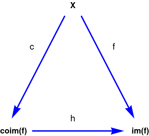
It is unique, because ker(c) = kerf, and it is an isomorphism, because the inverse mapping also exists and is defined uniquely. The point of uniting these spaces into pairs (with and without the prefix "co") is explained in the theory of duality.
In particular, if dimX = dimY = n < ∞, then for any linear operator f on X, indf = 0. This implies the so-called Fredholm alternative:
Theorem (Fredholm matrix Theorem): A system of linear algebraic equations A x = b has a solution if and only if b is orthogonal to every solution of the homogeneous equation z A = 0, that is, their inner p either the equation g(x) = y is solvable for all y and then the equation g(x) = 0 has only zero solutions; or this equation cannot be solved for all y and then the homogeneous equation g(x) = 0 has non-zero solutions. More precisely, if ind g = 0, then the dimension of the space of solutions of the homogeneous equation equals the codimension of the spaces on the right hand sides for which the inhomogeneous equation is solvable.
- Axler, Sheldon Jay (2015). Linear Algebra Done Right (3rd ed.). Springer. ISBN 978-3-319-11079-0.
- Halmos, Paul Richard (1974) [1958]. Finite-Dimensional Vector Spaces (2nd ed.). Springer. ISBN 0-387-90093-4.
- Katznelson, Yitzhak; Katznelson, Yonatan R. (2008). A (Terse) Introduction to Linear Algebra. American Mathematical Society. ISBN 978-0-8218-4419-9.
- Treil, S., Linear Algebra Done Wrong.
- Wikipedia, Dual space/