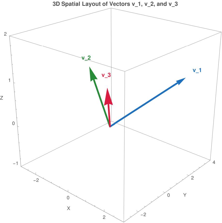
This block establishes how inner products allow us to define perpendicularity, angles, and structural decompositions in general vector spaces.
Orthogonality
In an abstract inner product space, we cannot use a physical protractor to measure a 90° angle. Instead, we use the algebra of the inner product to define a perfect right angle.
In a general inner product space (V, ⟨ • , • ⟩) over a field 𝔽 (ℝ or ℂ), two vectors x, y ∈ V
are said to be orthogonal (written as x ⊥ y) if and only if their inner product is exactly zero:
Example 2:
This example illustrates that orthogonality is not an intrinsic property of the vectors themselves, but a property dictated entirely by the choice of inner product.
Let x = [1, 1]ᵀ and y = [1, −2]ᵀ be vectors in ℝ².
1. Under the standard Euclidean dot product, they are clearly not orthogonal:
Thus, x and y
are completely orthogonal under this weighted inner product space.
■
End of Example 2
Example 3:
Moving away from finite coordinate arrays, this example shows how orthogonality applies to continuous functions where integration replaces summation.
Consider the vector space of real-valued continuous functions on the interval [−π , π], denoted ℭ([−π , π]), equipped with the standard functional inner product:
\[
\langle f , g \rangle = \int_{-\pi}^{\pi} \,f(x)\,g(x)\,{\text d}x .
\]
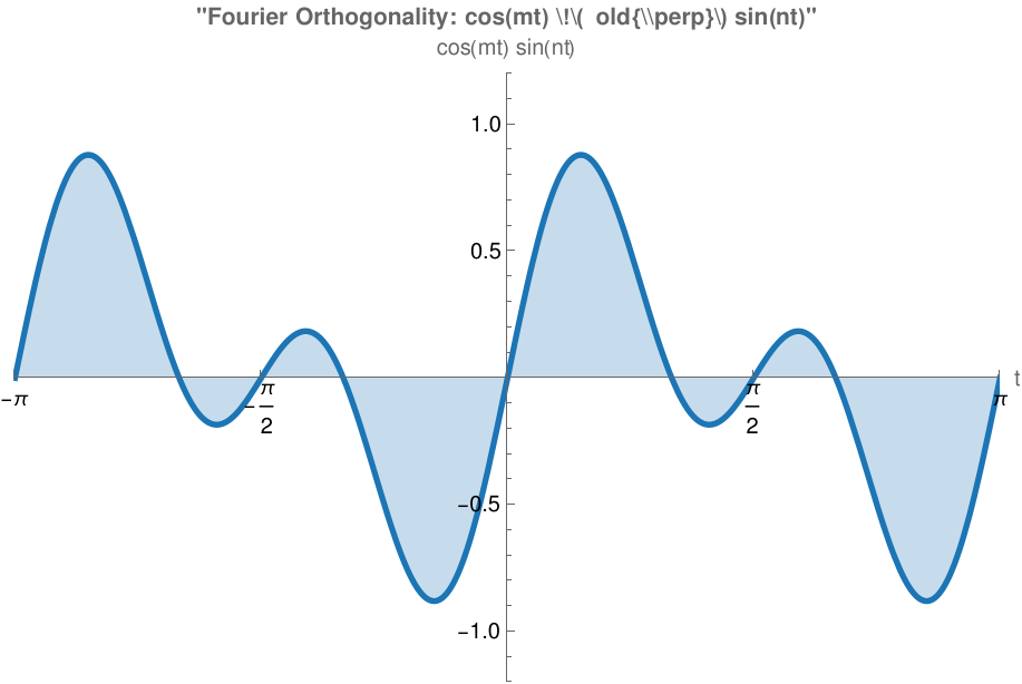
Let us verify that f(t) = cos(mt) and g(t) = cos(nt) are orthogonal for any integers m and n:
Using the trigonometric identity\( \displaystyle \quad \cos (A)\,\sin (B) = \frac{1}{2} \left[ \sin (A+B) - \sin (A-B) \right] , \quad \) the integrand becomes an odd function evaluated over a symmetric interval about zero:
This structural orthogonality forms the physical and mathematical foundation of Fourier series, where complicated signals are broken down into coordinates along a mutually perpendicular grid of sines and cosines.
Instead of varying an envelope width, this script allows you and your students to use interactive sliders to alter the integer frequencies m and n
for the functions f(t) = cos(mt) and g(t) = sin(nt) over the interval [−π , π].
(* Clear any existing definitions in the notebook context *)
ClearAll[fCos, gSin, fourierIntegrand];
(* 1. Explicitly define the basis functions accepting variable frequencies *)
fCos[t_, m_] := Cos[m*t];
gSin[t_, n_] := Sin[n*t];
fourierIntegrand[t_, m_, n_] := fCos[t, m] * gSin[t, n];
(* 2. Wrap the visualizer in an isolated, high-performance Manipulate frame *)
Manipulate[
Module[
{numericalInnerProduct},
(* Dynamically evaluate the functional inner product on [-π, π] *)
numericalInnerProduct = NIntegrate[
fourierIntegrand[t, mVal, nVal],
{t, -Pi, Pi},
Method -> "GlobalAdaptive"
];
(* Render the dynamic area cancellation plot *)
Plot[
fourierIntegrand[t, mVal, nVal],
{t, -Pi, Pi},
PlotStyle -> {Thickness[0.006], RGBColor[0.11, 0.46, 0.71]}, (* Royal Blue Curve *)
Filling -> Axis,
FillingStyle -> Directive[RGBColor[0.11, 0.46, 0.71], Opacity[0.25]],
PlotRange -> {{-Pi, Pi}, {-1.2, 1.2}},
Ticks -> {{-Pi, -Pi/2, 0, Pi/2, Pi}, Automatic},
AxesLabel -> {"t", "cos(mt) sin(nt)"},
LabelStyle -> Directive[FontFamily -> "Arial", FontSize -> 12],
PlotLegends -> Placed[
LineLegend[
{Row[{"Integrand Product with m = ", mVal, ", n = ", nVal}]},
LegendLabel -> Row[{"Functional Inner Product = ", StandardForm[Chop[numericalInnerProduct]]}]
],
Above
],
PlotLabel -> Style[
"Fourier Orthogonality: cos(mt) \!\(\bold{\perp}\) sin(nt)",
FontFamily -> "Arial", FontWeight -> Bold, FontSize -> 13
],
ImageSize -> 550
]
],
(* 3. Explicit discrete sliders to restrict m and n to integer frequencies *)
{{mVal, 1, "Frequency of Cosine (m)"}, 1, 6, 1, Appearance -> "Labeled"},
{{nVal, 2, "Frequency of Sine (n)"}, 1, 6, 1, Appearance -> "Labeled"}
]
Figure 3.1: Orthogonality of trig functions.
■
End of Example 3
Example 1:
This advanced example ties together a complex functional space, complex conjugates, and a non-trivial weight function—a setup standard in quantum mechanical wave mechanics.
Consider the complex inner product space of square-integrable functions equipped with a Gaussian weight function
over the real line
. The inner product is defined as:
\[
\langle f , g \rangle = \int_{-\infty}^{\infty} \,\overline{f(x)}\,g(x)\,e^{-x^2} \,{\text d}x .
\]
Let us test the orthogonality of a ground-state function f(x) = 1
and a complex first-excited-state component g(x) = x + ⅉx.
The term xe−x²
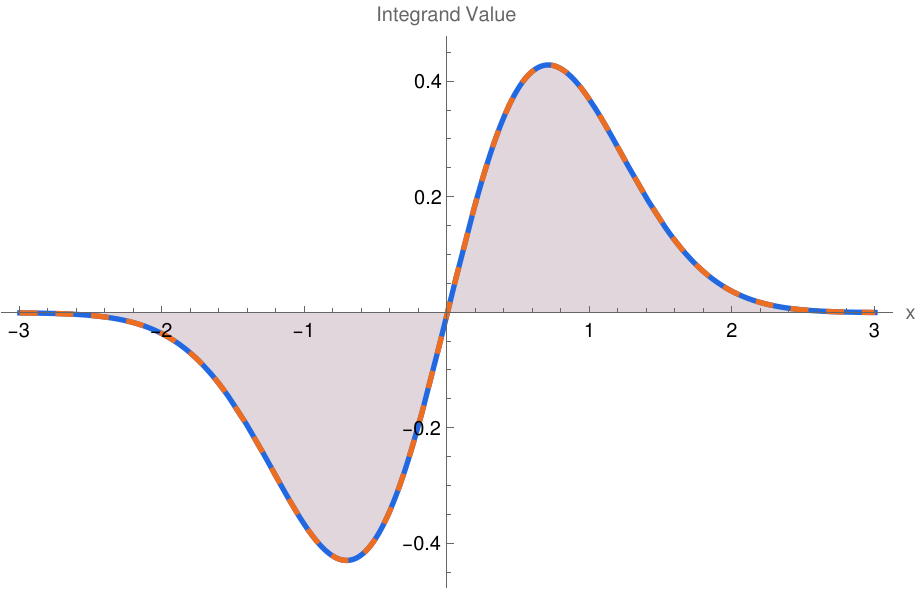
is an odd function. Because the limits of integration are completely symmetric from −∞ to ∞, the area under the curve cancels perfectly out to zero for both the real and imaginary parts:
\[
\langle f , g \rangle = 1(0) + \mathbf{j}(0) = 0 .
\]
Despite g(x) containing complex numbers and variable dimensions, these states are perfectly orthogonal under this specific Hilbert geometry.
Because the inner product of continuous functions is an integral, orthogonality means that the net accumulated area under the product of the functions (weighted by the Gaussian envelope) must cancel out to exactly zero. When working with a complex function g(x), this cancellation must happen independently for both the Real and Imaginary parts.
Below is the dynamic visualization followed by the production-ready Mathematica code to generate it. This Mathematica< script explicitly defines the complex inner product structure with the Gaussian weight, computes the analytical value to prove orthogonality, and outputs a publication-quality plot showing the area cancellation mechanism.
(* Clear any previous definitions in the workspace *)
ClearAll[weightW, fVec, gVec, weightedInnerProduct, integrandPlot];
(* 1. Define the Gaussian Weight Function and the State Functions *)
weightW[x_] := Exp[-x^2];
fVec[x_] := 1;
gVec[x_] := x + I*x;
(* 2. Compute the Analytical Inner Product over the Symmetric Infinite Domain *)
weightedInnerProduct = Integrate[Conjugate[fVec[x]] * gVec[x] * weightW[x], {x, -Infinity, Infinity}];
(* 3. Extract the Integrands explicitly as standard algebraic functions *)
realIntegrand[x_] := x * Exp[-x^2];
imagIntegrand[x_] := x * Exp[-x^2];
(* 4. Display Numerical Validation Results in Console *)
Print["=== QUANTUM MECHANICS ORTHOGONALITY CHECK ==="];
Print["Analytical Inner Product Result: ", weightedInnerProduct];
Print["Are the functional states orthogonal? ", weightedInnerProduct == 0];
(* 5. Generate Professional Textbook Visualization *)
integrandPlot = Plot[
{realIntegrand[x], imagIntegrand[x]},
{x, -3, 3},
PlotStyle -> {
{Thickness[0.006], RGBColor[0.13, 0.41, 0.88]}, (* Solid Blue line for Real Part *)
{Thickness[0.006], Dashing[{0.02, 0.02}], RGBColor[0.93, 0.43, 0.13]} (* Dashed Orange for Imag Part *)
},
Filling -> Axis,
FillingStyle -> {
1 -> Directive[RGBColor[0.13, 0.41, 0.88], Opacity[0.15]],
2 -> Directive[RGBColor[0.93, 0.43, 0.13], Opacity[0.15]]
},
AxesLabel -> {"x", "Integrand Value"},
LabelStyle -> Directive[FontFamily -> "Arial", FontSize -> 12],
PlotLegends -> Placed[
LineLegend[
{"Real Part: x exp(-x²)", "Imaginary Part: x exp(-x²)"},
LegendStyle -> Directive[FontSize -> 11]
],
Above
],
PlotRange -> All,
ImageSize -> 550
]
Figure 4.1: Area Cancellation in Complex Function.
As the plot highlights, both the real and imaginary curves exhibit perfect anti-symmetry (odd functions) across the origin. Every unit of negative area accumulated to the left of the y-axis (x < 0) is perfectly balanced by an identical unit of positive area to the right (x > 0), forcing the total inner product integral to collapse to zero.
To demonstrate how changing the Gaussian envelope width alters the geometry of your inner product space, we introduce a positive parameter σ
to govern the width. The modified inner product is defined as
\[
\langle f , g \rangle = \int_{-\infty}^{\infty} \,\overline{f(x)}\,g(x) \,e^{-x^2 /\sigma^2} \,{\text d}x .
\]
To make this fully interactive, we wrap the visualization in Mathematica's Manipulate function. This provides a real-time slider to change the scale
dynamically
Theorem 1:
If S = { v₁, v₂, … , vₙ } is an orthogonal set of non-zero vectors in an inner product space (V, ⟨ • , • ⟩), then S is linearly independent and hence is a basis for the subspace spanned by S.
To test for linear independence, set up the standard vector linear combination equal to zero:
Since vi
is a non-zero vector, its norm does not vanish, ∥vi∥ ≠ 0. Therefore, ci = 0. Because this holds true for every index i, all weights must be zero, proving linear independence.
Example 5:
This example demonstrates the necessity of the complex conjugate in the standard inner product on ℂ². Consider the vector space
equipped with the standard complex inner product \( \displaystyle \quad \langle \mathbf{x} , \mathbf{y} \rangle = x_1^{\ast} y_1 + x_2^{\ast} y_2 . \quad \) Let us verify that the following set is an orthogonal basis for ℂ²:
Because ⟨v , u⟩ = 0
and the vectors are non-zero, they form an orthogonal set. Since dim(ℂ²) = 2 and we have two linearly independent vectors, β
forms an orthogonal basis.
■
End of Example 5
When transitioning from ℝⁿ
to general and complex spaces, it should be emphasized these three critical upgrades:
The Inner Product Operator
In ℝⁿ: Orthogonality relies on the standard dot product (x • y = 0).
Orthogonality depends entirely on the specific inner product defined on that space (⟨x , y = 0).
The Complex Conjugate Subtlety.
In a complex inner product space, the inner product is conjugate-symmetric:
You should remember that if ⟨vi , vj⟩ = 0, its conjugate is also 0✶ = 0. Therefore, order does not matter when testing a basis for orthogonality; it remains a perfectly symmetric relation in ℂⁿ.
.
If we divide each vector in an orthogonal basis by its norm \( \displaystyle \quad \left( \mathbf{u}_i = \frac{\mathbf{v}_i}{\| \mathbf{v}_i \|}\right) , \quad \) we obtain an orthonormal basis, which is the gold standard for computational simplicity because the coordinate tracking equation collapses beautifully into:
Let (V, ⟨ • , • ⟩) be an inner product space over a field 𝔽 (where 𝔽 = ℝ or ℂ), and let W be a subspace of V. An orthogonal basis for W is a basis { v₁, v₂, … , vₙ } for W that is also an orthogonal set under the given inner product on V. That is, every vector in the set is non-zero, and orthogonal to all other vectors.
Example 2:
Theorem 2:
Let { v₁, v₂, … , vₙ }
Example 17:
■
End of Example 2
Let (V, ⟨ • , • ⟩)
be an inner product space over the field ℝ or ℂ. Two vectors v, u ∈ V
are said to be orthogonal (denoted as v ⊥ u) if and only if:
The Zero Vector Property: The zero vector 0
is the unique vector that is orthogonal to every vector in the space, since ⟨0 , v⟩ = 0
for all v ∈ V.
The Complex Symmetry Check: If v ⊥ u
in a complex space, then u ⊥ v
is automatically true because\( \displaystyle \quad \langle \mathbf{v} , \mathbf{u} \rangle = \overline{\langle \mathbf{u}, \mathbf{v} \rangle} = \langle \mathbf{u}, \mathbf{v} \rangle^{\ast} = \mathbf{0}^{\ast} = 0 . \quad \)
.
[Interactive Element Idea: A simple numerical widget where students input two complex coordinate pairs, and the site flashes green if their inner product equals zero.]
Section 2: Geometric Consequences
📘 Theorem 4: The Generalized Pythagorean Theorem
Theorem 2 (Generalized Pythagorean Theorem):
Let (V, ⟨ • , • ⟩) .
be an inner product space. If a set of vectors { v₁, v₂, … , vₙ }
is mutually orthogonal (meaning ⟨vi , vj⟩ = 0
whenever i ≠ j), then the squared norm of their sum is exactly equal to the sum of their individual squared norms:
Now consider a sum of n + 1
mutually orthogonal vectors. We can group the first n
vectors together as a single composite vector
\( \displaystyle \quad\mathbf{u} = \sum_{k=1}^n \,\mathbf{v}_k :\ \)
Insert the algebraic expansion and the induction scaffolding we finalized in our previous discussion here. Keeping this in an expandable accordion block keeps the main page from looking overly cluttered.]
🧪 Section 3: Nontrivial Application & Visual Proof
To prove to students that this geometry functions perfectly outside of basic arrow coordinates, include the infinite-dimensional calculus example.
📊 Continuous Waveforms Example
Let V = 𝔏²([−π , π])
with the standard integral inner product
. Let f(x) = sin(x) and g(x) = cos(x)
Section 4: Structural Frameworks
🧩 Orthogonal vs. Orthonormal Sets
When a grid of orthogonal vectors is scaled so that every single component has a standardized length of 1, it forms the ultimate coordinate system for computation.
Orthogonal Set: A collection of vectors where
for all
.
Orthonormal Set: An orthogonal set where every vector is a unit vector (
). This can be written compactly using the Kronecker Delta:
The Big Reward: Trivial Coordinate Extraction
Explain to students why we care about orthonormal bases (ONB). In a normal basis, finding the coordinates of a vector requires solving a massive system of linear equations (
). In an orthonormal basis, the inner product extracts coordinates instantly without any matrix inversion:
If{e_1
is an orthonormal basis for
, then any vector
can be written as:
Section 5: Algorithms & Future Steps
🔄 The Gram-Schmidt Process
An introductory teaser or link to the next subpage.
"What happens if our starting vectors are messy and not perpendicular? We use the Gram-Schmidt algorithm to systematically strip away the overlapping shadows (projections) until a pristine orthogonal framework is left behind."
🎓 Section 6: Quick Check Worksheet
Add 3 self-assessments at the bottom of the page so students can immediately test their comprehension before leaving the site.
True or False: If u ⊥ v, then ∥u − v∥² = ∥u∥² + ∥v∥². (Answer: True, the negative sign inside the norm vanishes under self-inner product expansion).
Dimension Check: Can an orthogonal set of non-zero vectors ever be linearly dependent? (Answer: No, orthogonality guarantees linear independence).
The Orthogonal Complement
When we have a subspace W
inside an inner product space (V, ⟨ • , • ⟩), we can cluster every single vector in the entire space that is perpendicular to W
into its own geometric structure.
Let W
be a subset (or subspace) of an inner product space (V, ⟨ • , • ⟩). The orthogonal complement of W, denoted by W⊥ (pronounced "W-perp"), is defined as:
Theorem 3:
Even if W
is just a random collection of scattered vectors, its orthogonal complement W⊥
is always a valid subspace of V.
.
Example 17:
■
End of Example 17
Theorem 4:
The only vector that can simultaneously live in a subspace and be perpendicular to itself is the zero vector:
\[
W \cap W^{\perp} = \{ \mathbf{0} \} .
\]
Example 18:
■
End of Example 18
Theorem 5:
If V is finite-dimensional and W is a subspace, then any vector in the universe V can be cleanly broken down into a "shadow" component in W and a perpendicular component in W⊥:
\[
V = W \oplus W^{\perp} \qquad\Longrightarrow\qquad \dim (V) = \dim (W) + \dim (W^{\perp}) .
\]