Since the tangent and normal vector fields, T(t(t) and N(t), were introduced in the previous section, respectively, to the
position vector field r(t) = 〈x(t), y(t), z(t), we might as well introduce one last
vector field. It was shown that the tangent and normal vector fields were orthogonal; therefore,
by the definition of the cross product, we can find a third vector field that is orthogonal to both, T(t(t) and N(t). This is how we define the binormal vector field B(t):
A TNB Frame (also known in differential geometry as the Frenet-Serret frame) is a moving coordinate system that travels along a continuous 3D space curve. It acts as a localized set of axes providing geometric intuition about how a curve twists and bends through space.
The three Unit vectors that form the TNB frame:
Tangent (T): The unit vector pointing in the direction of motion.
Normal (N): The unit vector pointing toward the center of curvature (where the curve is bending). It is perpendicular to T.
Binormal (B): The unit vector perpendicular to both, T
and N, computed via the cross product B = T × N.
In Mathematica, we can define the TNB frame symbolically for any vector-valued function r(t). Below is clean, vectorized code optimized for standard web formatting. We start with the Symbolic Definitions.
(* 1. Define the parametric curve *)
ClearAll[r, t, T, Nv, B];
r[t_] := {Cos[t], 2 Sin[t], t/2};
(* 2. Define the analytical TNB Frame vectors *)
T[t_] := Simplify[r'[t] / Norm[r'[t]], t ∈ Reals];
Nv[t_] := Simplify[T'[t] / Norm[T'[t]], t ∈ Reals];
B[t_] := Simplify[Cross[T[t], Nv[t]], t ∈ Reals];
(* 3. Evaluate the frame at a specific point (e.g., t0 = Pi/2) *)
t0 = Pi/2;
pos = r[t0];
tVec = T[t0];
nVec = Nv[t0];
bVec = B[t0];
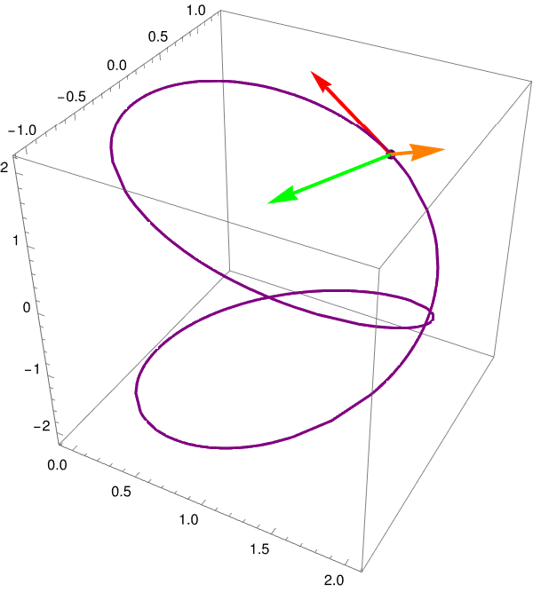
(* 4. Combine the space curve and vectors into a 3D Plot *)
Show[
(* Plot the continuous helix line *)
ParametricPlot3D[r[t], {t, 0, 3 Pi},
PlotStyle -> {Thick, Blue},
BoxRatios -> {1, 1, 1}],
(* Render the localized TNB coordinate system *)
Graphics3D[{
(* Tangent Vector - Red *)
Thickness[0.008], Red, Arrow[{pos, pos + tVec}],
(* Normal Vector - Green *)
Green, Arrow[{pos, pos + nVec}],
(* Binormal Vector - Orange *)
Orange, Arrow[{pos, pos + bVec}],
(* Position vertex dot *)
PointSize[0.02], Blue, Point[pos],
(* Structural text labels *)
Black,
Text[Style["T", 16, Bold, Red], pos + 1.25 tVec],
Text[Style["N", 16, Bold, Green], pos + 1.25 nVec],
Text[Style["B", 16, Bold, Darker[Orange]], pos + 1.25 bVec]
}],
PlotRange -> All,
AxesLabel -> {"X", "Y", "Z"},
ImageSize -> Large
]<
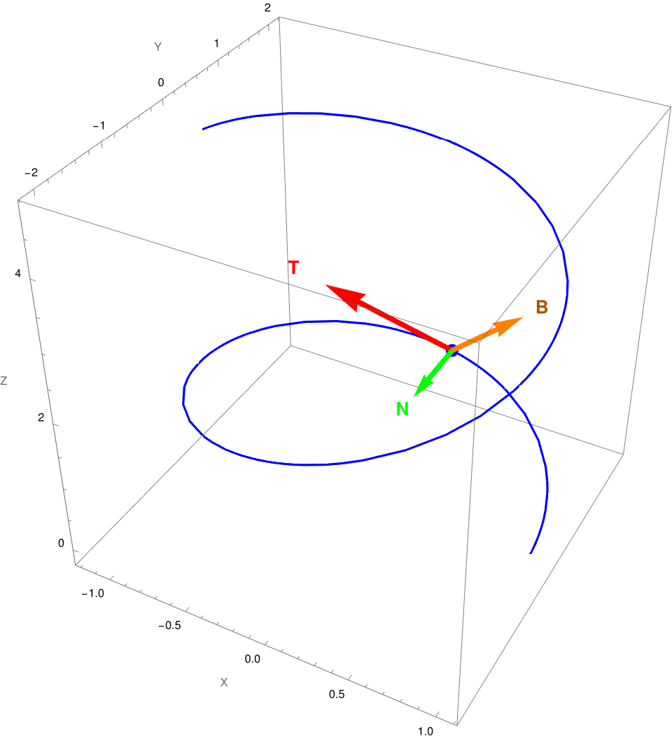
Figure 1: The TNB frame.
Note that since T(t) and N(t are unit vector fields, the binormal vector field is also a unit
vector. Remember that we have the formula
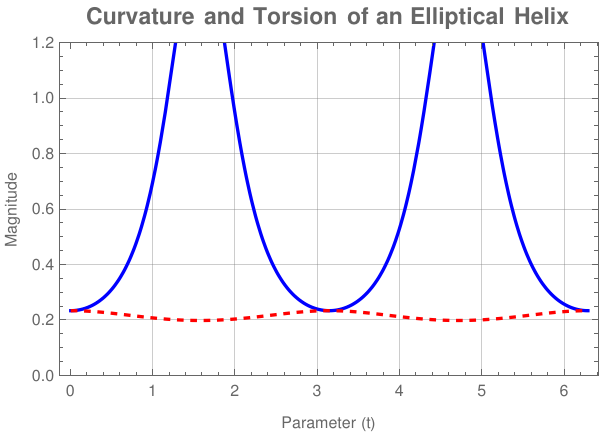
Unlike a standard circular helix (where curvature and torsion are both perfectly constant), an elliptical helix has a fluctuating curvature profile while maintaining a constant torsion.
(* 1. Define the parametric curve *)
ClearAll[r, t, curvature, torsion];
r[t_] := {Cos[t], 2 Sin[t], t/2};
(* 2. Define Curvature (Kappa) and Torsion (Tau) analytically *)
curvature[t_] := Simplify[Norm[Cross[r'[t], r''[t]]] / Norm[r'[t]]^3, t ∈ Reals];
torsion[t_] := Simplify[Dot[Cross[r'[t], r''[t]], r'''[t]] / Norm[Cross[r'[t], r''[t]]]^2, t ∈ Reals];
(* 3. Plot both metrics over a full period (0 to 2 Pi) *)
Plot[
{curvature[t], torsion[t]}, {t, 0, 2*Pi},
PlotStyle -> {{Thick, Blue}, {Thick, Red, Dashed}},
PlotRange -> {0, 1.2},
Frame -> True,
FrameLabel -> {"Parameter (t)", "Magnitude"},
PlotLegends -> LineLegend[
{Row[{Style["Curvature (", Plain], "κ", Style[")", Plain]}],
Row[{Style["Torsion (", Plain], "τ", Style[")", Plain]}]},
LegendStyle -> {FontSize -> 12}
],
PlotLabel -> Style["Curvature and Torsion of an Elliptical Helix", 14, Bold],
GridLines -> Automatic
]
Figure 1.2: Curvature and torsion of an elliptical helix.
■
End of Example 1
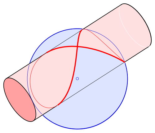
Example 2: Viviani's curve, also known as Viviani's window, is a figure-eight-shaped space curve named after the Italian mathematician Vincenzo Viviani (1622--1703).
Formed by intersecting a sphere with a cylinder, this closed loop showcases variable curvature and torsion profiles along its figure-eight trajectory.
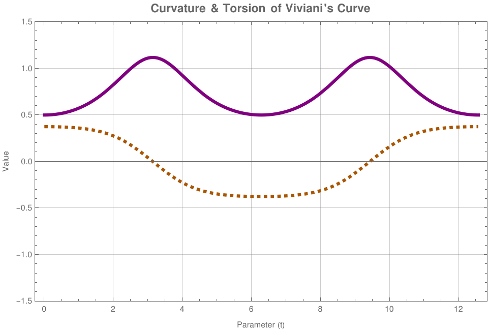
Because Viviani's curve forms a figure-eight loop on the surface of a sphere, both its curvature and torsion change dramatically as it approaches and passes through the central self-intersection point.
Figure 2.2: Curvature and torsion (in dashed) of Viviani's curve.
■
End of Example 2
Example 3:
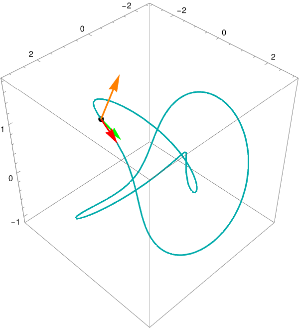
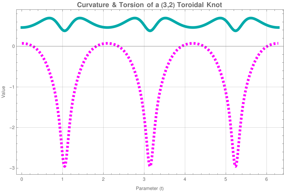
A curve wrapping tightly around a 3D torus geometry, demonstrating rich structural complexity ideal for stress-testing cross-product visualizations.
A toroidal knot wraps tightly around the surface of a torus, creating intricate, periodic variations in both how the curve bends and how it twists out of its local plane.
Figure 3.2: Curvature and torsion for a toroidal knot
■
End of Example 3
Differential Geometry of 3D Curves: The TNB Frame in Mathematica
A moving coordinate system traveling along a continuous 3D space curve is known as the Frenet-Serret frame, or more simply, the TNB Frame. The Frenet–Serret formulas describe the kinematic properties of a particle moving along a differentiable curve in three-dimensional Euclidean space ℝ³.
The TNB frame provides local intuition about how a curve bends, twists, and progresses through space by computing three mutually orthogonal unit vectors at any given point \(\vec{r}(t)\).
Mathematical Definitions & Numbered Relations
The TNB system is built sequentially. The primary direction is determined by the Unit Tangent Vector in Eq. \eqref{eq:tangent}, which tracks local velocity. From there, the local geometric bending yields the Unit Normal Vector defined in Eq. \eqref{eq:normal}. Together, they define a dynamic plane where the secondary metrics—the Binormal Vector in Eq. \eqref{eq:binormal}, Curvature in Eq. \eqref{eq:curvature}, and Torsion in Eq. \eqref{eq:torsion}—quantify spatial distortion.
Mathematica Tip: Because Mathematica treats variables as complex numbers by default, always evaluate your vectors using Simplify[..., t ∈ Reals]. This avoids unnecessarily complex expressions filled with absolute value wrappers (Abs).
Symbolic Framework Engine
Deploy this core engine in your Wolfram notebook to generate analytic formulas matching equations \eqref{eq:tangent} through \eqref{eq:torsion} for any parameterized curve:
Example 4:
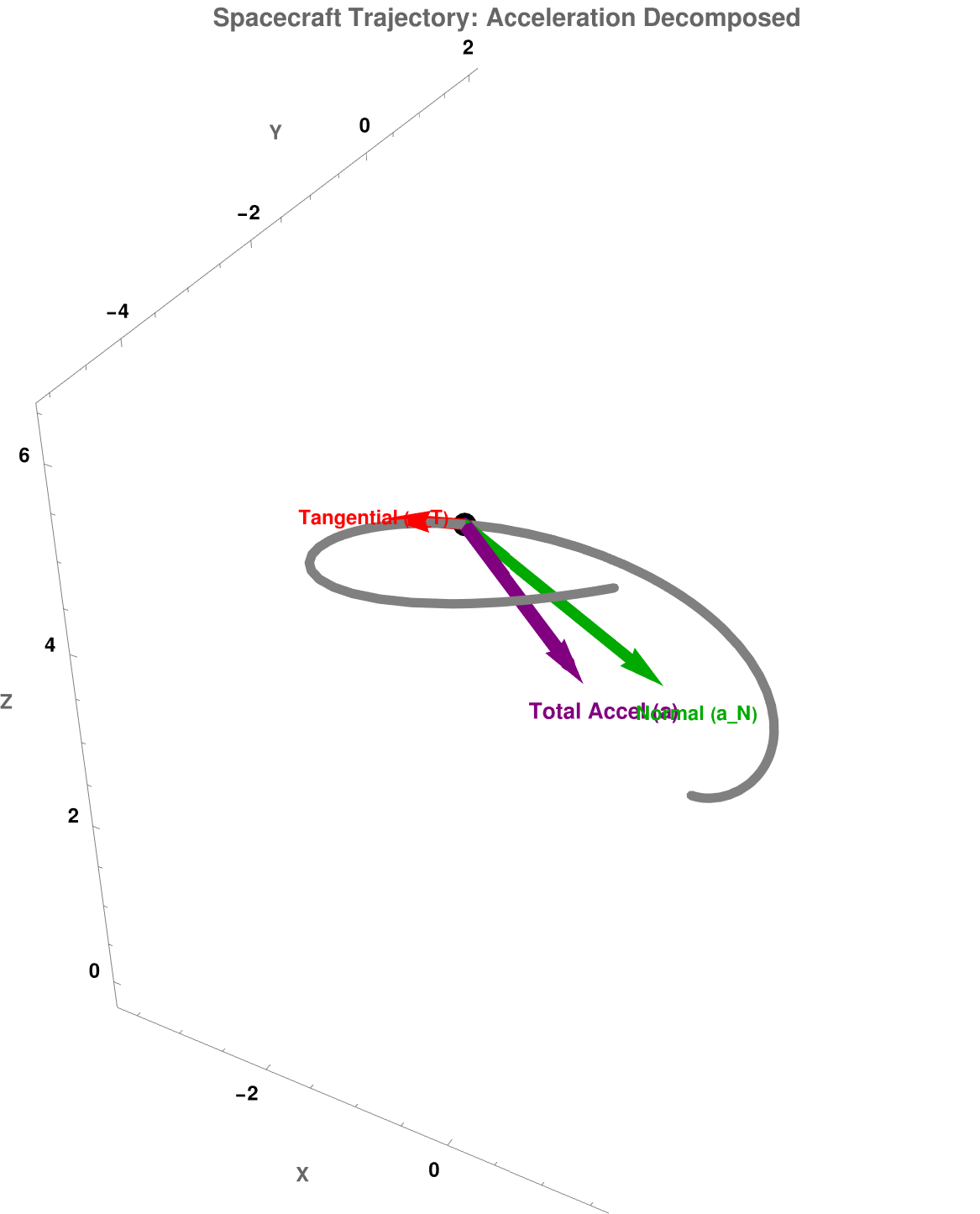
A highly elegant and nontrivial application of TNB frames is found in Aerospace Engineering and Physics: The Formulation of Rocket Trajectory Mechanics and G-Force (gravitational force) Tracking during High-Speed Maneuvers.
When a jet fighter or a rocket travels along a complex 3D flight path, analyzing its motion using standard fixed Cartesian coordinates
is incredibly inefficient. Instead, engineers map the vehicle's telemetry directly onto its moving TNB (Frenet-Serret) frame.
Tangential Acceleration points entirely along the Tangent vector (T). This component measures how much the vehicle's speed is changing (e.g., rocket engines firing or air brakes deploying).
Normal Acceleration points entirely along the Normal vector (N). This component measures how much the vehicle's direction is changing due to local curvature (κ).
There is zero acceleration along the Binormal vector (B). This mathematical absolute provides immense engineering utility:
The Osculating Plane: The vectors T and N
span a plane called the osculating plane. Because acceleration rests completely within this plane, the vehicle's instantaneous turning maneuver is always localized to a 2D slice of space.
Tracking Pilot G-Forces: The Binormal vector (B = T × N) acts as the dynamic axle of the turn. When an aircraft executes a sharp bank, the pilot experiences lateral forces. By evaluating Torsion (τ) along the flight path, aerospace software computes how fast the plane's plane-of-motion is twisting. This is used to ensure a missile or aircraft doesn't execute a maneuver that structurally tears its fuselage apart or causes a pilot to experience a fatal G-induced loss of consciousness (G-LOC, stands for G-force induced loss of consciousness}. It is a dangerous medical state where the brain is temporarily starved of oxygen (cerebral hypoxia) because high acceleration forces drain blood downward into the lower body).
Example 5:
n telecommunications engineering, long-haul fiber optic cables are rarely laid in straight lines. They must navigate subterranean conduits, twist around utility poles, or wind inside oceanic deployments. Additionally, multiple delicate glass fibers are spun into helical or planetary bundles within a single cable housing to allow for expansion and contraction.
A fiber optic cable consists of a pure silica core that transmits data via Total Internal Reflection (TIR). If a fiber is bent or twisted too aggressively, it suffers from two physical degradation mechanisms:
Macrobending Loss: Light leaks out of the core because the angle of incidence drops below the critical angle required for TIR.
Polarization Mode Dispersion (PMD): Physical twisting induces mechanical stress inside the glass cylinder, breaking its geometric symmetry. This creates birefringence, where different polarizations of light travel at different speeds, smearing the optical pulses and causing data corruption.
By mapping the path of the fiber using a moving TNB Frame, engineers precisely regulate these physical boundaries:
Curvature (κ) Limits: The radius of curvature R = 1/κ
cannot drop below the fiber's structural minimum bending radius. If κ
spikes, macrobending losses skyrocket.
Torsion (τ) Limits: Torsion measures how fast the Osculating Plane (spanned by T and N) rotates around the Tangent vector (T). This structural "twist rate" directly correlates with the torsional shear stress applied to the silica. Engineers use τ
to calculate the mechanical twist limits during the high-speed spinning process of manufacturing ribbon cables.
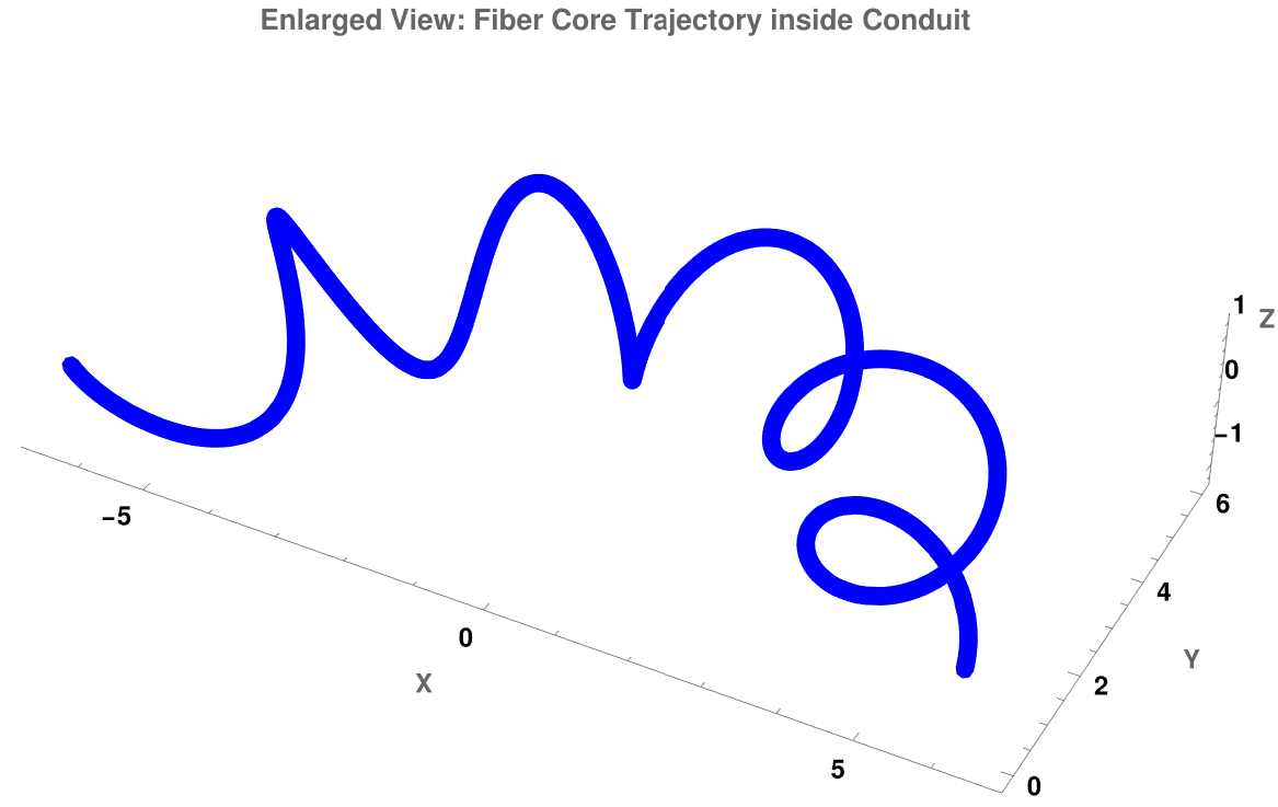
The following Mathematica code models a fiber optic thread spiraling inside a cable that is navigating a sweeping 3D bend. It extracts and displays the physical geometric stressors (κ and τ) along the path.
(* 1. Define updated, high-visibility geometry parameters *)
ClearAll[r, t, R, rCable];
R = 5; (* Radius of the main macro-bend conduit *)
rCable = 1.2; (* Enlarged internal spinning radius so it is highly visible *)
(* Parametric path of the fiber line winding inside the cable *)
r[t_] := {(R + rCable Cos[10 t]) Cos[t], (R + rCable Cos[10 t]) Sin[t], rCable Sin[10 t]};
(* 2. Generate an enlarged, thick 3D plot *)
ParametricPlot3D[
r[t], {t, 0, Pi},
PlotStyle -> {Directive[Thickness[0.015], Blue]}, (* Extra thick line style *)
PlotRange -> All,
Boxed -> False,
Axes -> True,
AxesLabel -> {"X", "Y", "Z"},
LabelStyle -> Directive[FontSize -> 14, Bold],
PlotLabel -> Style["Enlarged View: Fiber Core Trajectory inside Conduit", 16, Bold],
ImageSize -> 700 (* Maximized standalone display size *)
]
Figure 5.1: Fiber Core Trajectory.
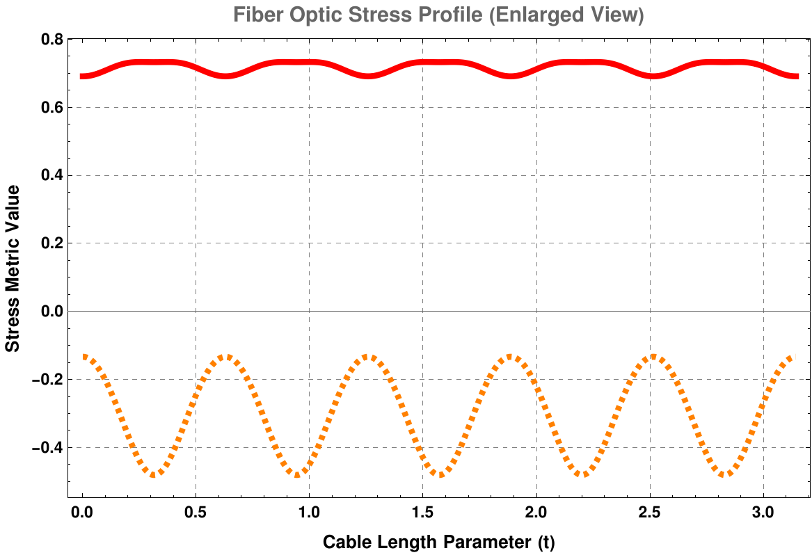
The code below provides enlarged, high-visibility 2D stress graph to complement the previous 3D plot.
Example 6:
In biophysics, the Frenet-Serret (TNB) Frame is the foundational mathematical framework used to describe the topological state, elastic energy, and mechanical supercoiling of double-stranded DNA molecules.
DNA (deoxyribonucleic acid) is the hereditary molecule that carries the genetic instructions used in the development, functioning, growth, and reproduction of all known living organisms
Inside a biological cell, DNA is not an unconstrained, relaxed ladder; it is packed under immense mechanical tension. When enzymes like RNA Polymerase track along the DNA to transcribe genes, they forcefully unwind the double helix ahead of them. This action introduces severe mechanical strain upstream and downstream, a phenomenon known as DNA Supercoiling.
To quantify this, biophysicists model the DNA backbone as a continuous space curve and apply the Călugăreanu-White-Fuller Theorem, which elegantly maps topological properties to the TNB frame parameters:
\[
Lk = Tw + Wr ,
\]
where
Linking Number (Lk): An invariant topological integer counting how many times the two strands intertwine. It can only change if a cell enzyme physically cuts the DNA backbone.
Twist (Tw): The local rotation of the DNA strands around the central axis. This is calculated directly by integrating the total torsion (τ) along the curve, combined with the normal vector rotation.
Writhe (Wr): A measure of the non-local, spatial coiling of the central axis itself (how the DNA loops over itself like an old telephone cord). Writhe is governed strictly by the curvature (κ) profile and non-local geometry.
If a cell cannot manage these parameters, the local Torsion (τ) builds up so heavily that the DNA molecule undergoes a phase transition—either buckling into a twisted knot (plectoneme, which is a structural motif where a double-stranded molecule—most commonly DNA—is wound around itself in a tight, rope-like helix) or ripping its base pairs apart. This stops all cellular life, which is why modern chemotherapies and antibiotics target topoisomerase enzymes to intentionally break this mechanical equilibrium.
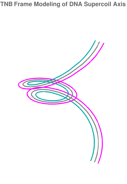
The following Mathematica code surves to Visualize DNA Supercoiling Energy:
(* 1. Model a supercoiled DNA plectoneme backbone loop *)
ClearAll[dnaCurve, t];
dnaCurve[t_] := {
(2 + Cos[t]) Cos[2 t],
(2 + Cos[t]) Sin[2 t],
5 t/Pi + 2 Sin[t]
};
(* 2. Generate the 3D molecular ribbon using the TNB system *)
T[t_] := Simplify[dnaCurve'[t] / Norm[dnaCurve'[t]], t ∈ Reals];
Nv[t_] := Simplify[T'[t] / Norm[T'[t]], t ∈ Reals];
(* Build a structural double-ribbon representing the two sugar-phosphate backbones *)
Show[
(* Main space axis *)
ParametricPlot3D[dnaCurve[t], {t, 0, 2 Pi}, PlotStyle -> {Thickness[0.01], Gray}],
(* Strand 1 (shifted along Normal vector) *)
ParametricPlot3D[dnaCurve[t] + 0.3 Nv[t], {t, 0, 2 Pi}, PlotStyle -> {Thickness[0.01], Darker[Cyan]}],
(* Strand 2 (shifted opposite to Normal vector) *)
ParametricPlot3D[dnaCurve[t] - 0.3 Nv[t], {t, 0, 2 Pi}, PlotStyle -> {Thickness[0.01], Magenta}],
PlotRange -> All,
Boxed -> False,
Axes -> False,
PlotLabel -> Style["TNB Frame Modeling of DNA Supercoil Axis", 14, Bold]
]
Figure 6.1: DNA starnd.
In biophysics and structural engineering, a thin rod (like a DNA strand or a fiber optic line) has a total Elastic Strain Energy (E) modeled by the Kirchhoff rod theory developed by Gustav Kirchhoff in 1859. It is a classical continuum mechanics model that describes the 3D bending and twisting of slender, elastic rods or beams (such as cables, hairs, or structural beams) where length is much greater than radius (ℓ > r).
By mapping the deformation to the curve's Curvature (κ) and Torsion (τ), the global mechanical energy is given by:
B is the Torsional/Twisting Stiffness Coefficient (governed by Shear Modulus).
τ₀ is the intrinsic torsion of the material when completely relaxed (e.g., the natural twist rate of DNA base pairs).
A physical system fails or buckles when these local values cross structural thresholds:
Bending Yield Point (κmax): Exceeding this causes micro-fractures in glass fibers or ruptures base-pair bonds in DNA.
Torsional Buckling Instability (τmax): When a thread accumulates too much torsion, it undergoes a geometric phase transition called writhing—buckling directly into a tight plectonemic loop to lower its twist energy.
The following unified script simulates a complex space curve trajectory, computes its local curvature and torsion, pinpointing where mechanical limits are exceeded via automated visual alerts, and then performs numerical integration to output the exact total elastic energy of the system.
(* 1. Define Trajectory System and Engineering Parameters *)
ClearAll[r, t, s, curvature, torsion, totalEnergy, bendingEnergy, twistingEnergy];
(* A complex spatial winding path *)
r[t_] := {Cos[3 t] (2 + Cos[t]), Sin[3 t] (2 + Cos[t]), 1.5 t + Sin[t]};
(* Material Constants (Adjustable values for structural modeling) *)
A = 100.0; (* Bending stiffness index *)
B = 80.0; (* Torsional stiffness index *)
tau0 = 0.2; (* Relaxed intrinsic torsion *)
(* Safety Thresholds *)
kappaMax = 1.1; (* Max safe curvature before fracture/disruption *)
tauMax = 0.5; (* Max safe torsion before twisting failure *)
(* 2. Analytical Curve Calculators *)
speed[t_] := Norm[r'[t]];
curvature[t_] := Simplify[Norm[Cross[r'[t], r''[t]]] / speed[t]^3, t ∈ Reals];
torsion[t_] := Simplify[Dot[Cross[r'[t], r''[t]], r'''[t]] / Norm[Cross[r'[t], r''[t]]]^2, t ∈ Reals];
(* 3. Compute Local Energy Density Functions *)
bendingDensity[t_] := (1/2) * A * (curvature[t]^2) * speed[t];
twistingDensity[t_] := (1/2) * B * ((torsion[t] - tau0)^2) * speed[t];
(* 4. Numerical Integration for Global Totals over the domain [0, 2Pi] *)
Print[Style["--- Global Energy Report ---", Bold, 14]];
totalBending = NIntegrate[bendingDensity[t], {t, 0, 2 Pi}];
totalTwisting = NIntegrate[twistingDensity[t], {t, 0, 2 Pi}];
Print["Total Bending Strain Energy: ", totalBending, " Joules"];
Print["Total Twisting Strain Energy: ", totalTwisting, " Joules"];
Print["Total Combined Elastic Energy: ", totalBending + totalTwisting, " Joules\n"];
(* 5. Diagnostic Plot: Highlighting Failure Points *)
Print[Style["--- Mechanical Structural Health Analysis ---", Bold, 14]];
Plot[
{curvature[t], torsion[t]}, {t, 0, 2 Pi},
PlotStyle -> {{Thick, Blue}, {Thick, Orange}},
Frame -> True,
FrameLabel -> {"Parameter (t)", "Value"},
PlotLegends -> {"Curvature (\[Kappa])", "Torsion (\[Tau])"},
PlotLabel -> "Local Spatial Stressors vs Material Limits",
GridLines -> Automatic,
ImageSize -> Large,
(* Inject visual safety boundaries into the background *)
Prolog -> {
(* Red alert region for excessive curvature *)
Opacity[0.15], Red, Rectangle[{0, kappaMax}, {2 Pi, 3.0}],
(* Orange alert region for excessive torsion *)
Opacity[0.15], Orange, Rectangle[{0, tauMax}, {2 Pi, 3.0}],
(* Label lines for clarity *)
Opacity[0.5], Darker[Red], Dashed, InfiniteLine[{0, kappaMax}, {1, 0}],
Darker[Orange], Dashed, InfiniteLine[{0, tauMax}, {1, 0}]
},
Epilog -> {
Text[Style["Curvature Failure Boundary", 10, Bold, Darker[Red]], {1, kappaMax + 0.05}, {-1, 0}],
Text[Style["Torsional Buckling Limit", 10, Bold, Darker[Orange]], {1, tauMax - 0.05}, {-1, 0}]
}
]
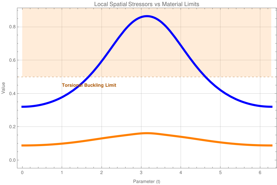
Figure 6.2: Curvature Failure Boundary.
The graph dynamically highlights stress envelopes in soft red and orange. Any part of the solid lines poking up into these colored blocks represents physical coordinates along the strand that are at risk of material failure.
Notice that during integration, the density equations are multiplied by speed[t] (which represents ds/dt). This converts parameter integration directly into physical arc-length integration seamlessly, keeping calculations geometrically precise regardless of how fast or slow the curve's parametrization is pacing.
■
End of Example 6
Plot the TNB frame for the spacecurve given by r(t) = [t, t cos(3t), t sin(3t)] with 0 ≤ t ≤ 4π.
Plot the TNB frame for the spacecurve given by r(t) = [cos(2 t), sin(3 t), cos(3 t)] with 0 ≤ t ≤ 4π.
Plot the TNB frame for the spacecurve given by r(t) = [(2 + cos(2t)) cos(3t), (2 + cos(2t)) sin(3t), sin(4t)] with 0 ≤ t ≤ 3π.
The following space curve lies on a torus and is given by r(t) = [(3 + 2 cos(t)) cos(10t), (3 + 2 cos(t)) sin(10t), 2 sin(t)] with 0 ≤ t ≤ 2π. Plot, in the same figure, the following graphs: r(t), the TNB frame for r(t), and the torus, given parametrically by s(u, v) = [(3 + 2 cos(v)) cos(u), (3 + 2 cos(v)) sin(u), 2 sin(v)], for −π ≤ u, v ≤ π.
The space curve r(t) = [(3 + 2 cos(3t)) cos(7t), (3 + 2 cos(3t)) sin(7t), 2 sin(3t)] for 0 ≤ t ≤ 2π, also lies on a torus given parametrically by s(u, v) = [(3 + 2 cos(v)) cos(u), (3 + 2 cos(v)) sin(u), 2 sin(v)], for −π ≤ u, v ≤ π. Plot, in the same figure, r(t), the TNB frame for r(t), and the torus.
Plot the curvature function κ(t) for the space curve from the previous problklem.
Consider the standard circular helix parametrized by r(t) = [𝑎 cos(t), 𝑎 sin(t), bt], where 𝑎 > 0 and b > 0 are constants.
Find the unit tangent vector T(t).
Find the principal normal vector N(t)
and show that it always points directly toward the z-axis.
Compute the binormal vector B(t).
Show that both the curvature κ(t) and torsion τ(t) are completely constant for all t.
Let r(t) = [t, t², 0] be a parabola constrained to the xy-plane.
Compute the TNB frame vectors at the vertex t = 0.
Calculate the torsion τ(t) for any arbitrary t.
Conceptual question: What must the torsion always be for any curve that lies completely flat within a single plane? Why?
A drone is tracking a path modeled by \( \displaystyle \quad \mathbf{r}(t) = \left[ e^t , \ \sqrt{2}\,t, \ e^{-t} \right] . \)
Compute the velocity vector v(t) and the acceleration vector 𝑎(t).
Decompose the acceleration vector into its tangential component (𝑎T(t)) and normal component (𝑎N(t)) such that 𝑎 = 𝑎TT + 𝑎NN.
If the drone's structural hull fails when the directional bending acceleration (
𝑎N) exceeds 2.0 m/s², determine if the drone survives its maneuver at t = 0.
An engineer is pulling a fiber optic cable through a curved machine guide. The line's trajectory follows Viviani's curve r(t) = [1 + cost, sint, 2 sin(t/2)]
Find the points along the interval t ∈ [0, 4π]
where the torsion τ(t) = 0.
Explain what is happening to the moving osculating plane at these exact coordinates. Is the fiber twisting or momentarily flattening out?
Write a script to calculate and plot the curvature κ(t) and torsion τ(t) side-by-side for t ∈ [0, 2π].
By inspecting your generated graphs, visually identify how many distinct curvature "peaks" (local maxima) occur over one full revolution. What physical geometric property of the torus causes this oscillation?
Calladine, C. R., Drew, H. R., Luisi, B. F., & Travers, A. A. (2004). Understanding DNA: The Molecule and How it Works (3rd ed.). Academic Press.
Do Carmo, M. P. (2016). Differential Geometry of Curves and Surfaces (2nd ed.). Dover Publications.
Ghatak, A., & Thyagarajan, K. (1998). Introduction to Fiber Optics. Cambridge University Press.
Greenwood, D. T. (1988). Principles of Dynamics (2nd ed.). Prentice Hall.
Stewart, J. (2020). Calculus: Early Transcendentals (9th ed.). Cengage Learning.
White, J. H. (1969). Self-linking and the Gauss integral in higher dimensions. American Journal of Mathematics, 91(3), 693-728.