This section is devoted to basic manipulations with matrices that have only two dimensions: rows ×
columns, or matrices that you could print out and lay flat on a
table.
Although the number of dimensions in which a matrix lives is more
open to interpretation compared to what we use in this section, matrices in higher dimensions (say that would require a 3D printer) could be found elsewhere. We discuss later matrices
in physical space, which are called tensors.
Matrices are ubiquitous in mathematics, physics, and engineering because
of their diverse intentions. To give you an idea of their
versatility, below is a non-exhaustive list of some applications of matrices.
Representing a linear transformation or mapping;
Using as operators acting on vectors;
Representing a system of equations;
Storing data (e.g., features × observations);
Storing kernels used in filtering or convolution;
Representing finance information from different sectors of
an economy or business;
Deriving parameters for a model that predicts changes in the
spread of an infectious disease.
When referring to matrix sizes, and when referring to indices in a
matrix, it is assumed that you refer first to rows then to columns. When a matrix has m rows and n columns, we speak about m-by-n or m × n matrix; so this matrix has two dimensions, and we call it m × n or (m, n).
An m-by-nmatrix is a rectangular array or list of lists containing numbers, symbols, expressions, or algebraic objects, arranged in m rows and n columns.
There are two common notations for matrices, either in square brackets or parentheses. For example,
Note: Since matrices can be considered as operators acting on either column vectors from left or on row vectors from right, we use bracket notation for latter and embrace matrices in parentheses when they act on row vectors from right.
■
Although entries of a matrix could be arbitrary algebraic objects, we consider in this section only naïve entries that belong to one of the following fields: set of integers, ℤ, or rational numbers, ℚ, or real numbers, ℝ, or complex numbers, ℂ. The set of all m × n matrices over field 𝔽 is denoted by 𝔽m×n. We use capital bold letters, such as A or M, to denote matrices.
Since mathematica does not display naturally (for humans) matrices, it is convenient to force this software package to do this job for you by entering the following code:
The element in the i-th
row, j-th column in matrix A is denoted A[i, j] or Ai, j or 𝑎i, j if A = [𝑎i, j].
There is no standard notation for specifying a particular row or column
of a matrix. Following matlab, we use the notation A[i, :] for the i-th row of A
(a row vector) and A[: , j] for the j-th column. (matlab uses parentheses rather
than square brackets, however). Mathematica uses notation A[i, j] for (i, j) element of matrix A, but notation for extracting corresponding rows or columns will be given later.
Linear Combinations of Matrices
We show that matrices of the same size form a vector space.
Algebraically, matrices can be added and scalar-multiplied, just like vectors,
numeric and geometric vectors.
The sumC = [ci, j] of two m × n
matrices A = [𝑎i, j] and B = [bi, j] is again an m × n matrix. We get its
entries from the simple rule ci, j = 𝑎i, j + bi, j. Addition requires that both
matrices have the same size (the same numbers of rows and columns).
The difference of two m × n
matrices A = [𝑎i, j] and B = [bi, j] is the m × n matrix D = [di, j] with entries di, j = 𝑎i, j − bi, j.
Observation 1:
Matrix addition is commutative and associative:
For any matrices A, B, and C of the same size, we have
\[
{\bf A} + {\bf B} = {\bf B} + {\bf A} , \qquad {\bf A} + \left( {\bf B} + {\bf C} \right) = \left( {\bf A} + {\bf B} \right) + {\bf C} .
\]
The product of a
matrix A = [𝑎i, j] with a scalar r is denoted by rA or Ar. The entry in row
i, column j of rA is simply
r 𝑎i, j, so that rA = [r 𝑎i, j].
To multiply matrix A by a scalar (number) r ∈ 𝔽 (either from the left or from the right), just
multiply every element of the matrix by the number (scalar):
for some scalars c₁, c₂, … , ck and some matrices A₁, A₂, … , Ak of the same size. Then this linear combination is again a matrix of the same size. This means that the set 𝔽m×n of all m × n matrices is a vector space.
Furthermore, the above operations are also distributive in two senses. On the one
hand, you can push the same matrix A into parentheses:
Observation 2:
For every m × n matrix A ∈ 𝔽m×n,
there is a unique m × n matrix M such that
A + M = A. This matrix is called the zero matrix and it is denoted by 0.
Observation 3:
For every m × n matrix A ∈ 𝔽m×n,
there is a unique m × n matrix M such that
A + M = 0. This matrix is called the additive inverse of A and it is denoted by −A.
A ={{1,2,3,4},{4,-3,2,-1},{1,-1,1,-1}};
B ={{2,1,3,1},{3,-2,1,-2},{4,-2,3,-3}};
A + B
{{3, 3, 6, 5}, {7, -5, 3, -3}, {5, -3, 4, -4}}
A - B
{{-1, 1, 0, 3}, {1, -1, 1, 1}, {-3, 1, -2, 2}}
A linear combination of these two matrices, for instance, is
\[
2\,{\bf A} -3\, {\bf B} = \begin{bmatrix} -4& 1& -3& 5 \\ -1& 0& \phantom{-}1& 4 \\ -10& 4& -7& 7 \end{bmatrix} .
\]
2*A -3*B
{{-4, 1, -3, 5}, {-1, 0, 1, 4}, {-10, 4, -7, 7}}
■
End of Example 1
Matrix times Vector---Operator
In the computer algebra system Mathematica, a matrix is considered a list of lists. In case of our naïve definition of matrices, this list is filled with scalars from field 𝔽, either ℤ (which is preferred by the laziest people in academia, like me), integers, or ℚ, the rational numbers, ℝ, the real numbers, or ℂ, the set of complex numbers. Therefore, an m-by-n matrix can be considered as a list of m rows:
Here δi,j is the Kronecker delta.
To define a product A x of vector x = (x₁. x₂, … , xn) by matrix A = [𝑎i, j] from left, we need two things. First, we need to convert vector x ∈ 𝔽n from n-tuple into column vectors from 𝔽n×1. This transformation is essential for matrix multiplication from left. Otherwise, you use vector/matrix multiplication for matrix acting on vector x from right; in this case, you need to convert the n-tuple vector into row vector. Since these three vector spaces, 𝔽n (Cartesian product of n copies of field 𝔽), 𝔽n×1 (space of column vectors), and 𝔽1×n (space of row vectors), are isomorphic, 𝔽n ≌ 𝔽n×1 ≌ 𝔽1×n, there exists a one-to-one and onto linear mapping that transfers one space into another.
Second, we need
a special notation that abbreviates specific calculations.
The dot product of two n-dimensional vectors from 𝔽n is computed by multiplying corresponding components, and then adding all these products. That is,
where x = (x₁. x₂, … , xn), y = (y₁. y₂, … , yn) ∈ 𝔽n.
We indicate it by a large solid dot, •, because it has many different purposes of applications, not only in matrix/vector multiplication. The dot product is not defined for vectors of different dimensions.
Note: Although dot product defines a metric (distance) in real spaces, it has some weird properties in complex spaces; for instance, (1, j) • (1, j) = 0, where j is the imaginary unit in complex plane ℂ, so j² = −1. Therefore, the dot product is not suitable for metric definition in complex spaces--there is an inner product instead. So we use dot product in complex spaces only formally, as a short-cut for linear combinations. ■
When written this way, we can use the “two-hands" method to compute
the product: the left hand moves from left to right along each row of the matrix
while the right hand moves from top to bottom along the column vector.
where cj(A) = A eTj = A[:, j] is the j-th column of matrix A, j = 1, 2, … , n. here eTj is column vector obtained from row vector ej by writing it vertically (T indicates transposition). This way, each column of A is in 𝔽m×1. Let us consider now a different column vector, not in 𝔽m×1 but rather in 𝔽n×1:
Since there are exactly n components in matrix A representation via columns, we can now scan A column by column, multiplying each column by the corresponding component from vector x, and sum up
This indeed represents A x as a linear combination of the columns of A, with coefficients taken as components of vector x. Hence, matrix multiplication defines a linear transformation:
because 𝔽n×1 is isomorphic to 𝔽n. Such multiplication of matrix and column vector given in Eq,(3) is called matrix/vector operation, or more precisely, matrix/column multiplication.
We can also define a dual multiplication on a vector from right If y = [y₁, y₂, … , ym] ∈ 𝔽1×m is a row vector of length m, we define its product with m×n matrix A as follows:
This rule (4) is known as vector/matrix operation or more precisely, row/matrix multiplication.
Observation 4:
Every m × n matrix defines a linear transformation 𝔽n×1 ⇾ 𝔽m×1 with mapping column vector x into column vector A x upon multiplication from left by matrix A.
Similarly, this matrix acts on row vectors y of size m via multiplication from right, transferring it into row vectors y A of size n.
The important features of matrix/vector and vector/matrix
multiplications are that they provide the connection between
linear transformations and matrices: To apply a transform to a
vector, you convert that transform into a matrix, and then you
multiply the vector by that matrix, either from left considering vector as a column or from right representing a vector as a row. Multiplying m-by-n matrix A by vector x depends on the size pf the vector. If x has length n, then you have to convert it into column vector and multiply matrix A from left. However, if x ∈ 𝔽m, then you have no choice as to consider this vector as a row and multiply matrix A from right.
You can always convert column vectors into rows and vice versa by using transposition operation (see below) because
Example 2:
We consider a rectangular matrix
\[
{\bf A} = \begin{bmatrix} 2&3&-1&\phantom{-}2 \\ 5&1&-3&-2 \\ 4&2&-3&-1 \end{bmatrix} .
\]
Upon multiplying it on row vector from right, we get
\[
\begin{bmatrix} 2& -3& 5 \end{bmatrix} \begin{bmatrix} 2&3&-1&\phantom{-}2 \\ 5&1&-3&-2 \\ 4&2&-3&-1 \end{bmatrix} = \begin{bmatrix} 9 & 13 & -8 & 5 \end{bmatrix} .
\]
Clear[A, B, x, y];
A = {{2, 3, -1, 2}, { 5, 1, -3, -2}, { 4, 2, -3, -1}};
y = {2, -3, 5};
y . A
{9, 13, -8, 5}
On the other hand, multiplying matrix A by column vector from left, we obtain
\[
\begin{bmatrix} 2&3&-1&\phantom{-}2 \\ 5&1&-3&-2 \\ 4&2&-3&-1 \end{bmatrix} \cdot \begin{bmatrix} -1 \\ \phantom{-}2 \\ \phantom{-}3 \\ -4 \end{bmatrix} = \begin{bmatrix} -7\\ -4 \\ -5 \end{bmatrix} .
\]
x = {-1 , 2 , 3 , -4};
A.x
{-7, -4, -5}
■
End of Example 2
Example 3:
According to the USDA, 100 grams of watermelon contains
Calories: 30 Kcal
Carbs: 7.6 grams
Sugar: 6.2 grams
Protein: 0.6 grams
Potassium: 0.17 grams
Fiber: 0.6 grams
100 grams of strawberries contains
Calories: 32 Kcal
Sugar: 4.89 grams
Protein: 0.67 grams
Potassium: 0.153 grams
Magnesium: 0.013 grams
Fiber: 2 grams
100 grams of kiwi contains
Calories: 61 Kcal
Sugar: 8.99 grams
Protein: 1.14 grams.
Potassium: 0.312 grams.
Magnesium: 0.017 grams.
Fiber: 3 grams.
If one eats w kg of watermelon, s kg of strawberries, and k kg of kiwi, then the amount of protein p, the amount of fiber f, and the
amount of sugar s they will have consumed is given by the system of linear equations
\begin{align*}
0.6\,w + 0.67\, s + 1.14\,k &= 10\,p ,
\\
0.6\,w + 2\,s + 3\,k &= 10\,f ,
\\
6.2\, w + 4.89\,s + 8.99\, k &= 10\, s .
\end{align*}
We can rewrite this system in matrix/vector form:
\[
\begin{bmatrix} 0.6 & 0,67 & 1.14 \\ 0.6 & 2 & 3 \\ 5.2 & 4.89 & 8.99 \end{bmatrix} \cdot \begin{bmatrix} w \\ s \\ k \end{bmatrix} = 10 \begin{bmatrix} p \\ f \\ s \end{bmatrix} .
\]
Observe that we can write the amount of protein being consumed as the dot product
\[
p = 0.1 \left[ 0.6 \ 0.67 \ 1.14 \right] \bullet \left[ w \ s \ k \right] .
\]
Example 4:
Let us consider 2 × 2 matrix, which is multiplied by a vector from left and right:
\[
\begin{bmatrix} a&b \\ c&d \end{bmatrix} \cdot \begin{bmatrix} x \\ y \end{bmatrix} = \begin{bmatrix} a\,x + b\,y \\ c\,x + d\,y \end{bmatrix}
\]
Clear[a,b,c,d,x,y]
A = {{a, b}, {c, d}};
A . {x, y}
{a x + b y, c x + d y}
On the other hand,
\[
\begin{bmatrix} x & y \end{bmatrix} \cdot \begin{bmatrix} a&b \\ c&d \end{bmatrix} = \begin{bmatrix} a\,x + c\,y \\ b\,x + d\,y \end{bmatrix}
\]
{x, y} . A
{a x + c y, b x + d y}
These mathematica scripts confirm that this computer algebra system is very smart and it knows when apply column vector and when row vector!!
So we conclude that these two matrix.vector products match only when matrix A is symmetric: A = AT, i.e., b = c,
■
End of Example 4
Matrix times Matrix
Before learning how (standard) matrix multiplication works,
the first thing you need to know about this topic is that the matrix product exists only for compatible matrices: when matrix A is multiplied by matrix B from right, their dimensions must match. In other words the number of columns in matrix A should be equal to the number of rows in matrix B in order for the product A B to exist. Therefore, the existence of product A B does not guarantee that reverse product B A exists; but when both products hold true, it is commutative only in rare cases and generally speaking A B ≠ B A.
The following five statements provide useful terminology for saying that product A B is valid for matrices A and B:
A times B (which is denoted by A B),
A pre-multiplies B,
A left-multiplies B,
B right-multiplies A
B post-multiplies A.
There are four ways to implement matrix multiplication of two matrices that provide insights
into matrix computations in different contexts and for different
problems. We denote by C [ci,j] the product of two matrices
Example 5:
We consider the product of two matrices
\[
{\bf A}_{3 \times 2} = \begin{bmatrix} 0&1 \\ 2&3 \\ 4&5 \end{bmatrix} , \qquad {\bf B}_{2 \times 2} = \begin{bmatrix} a&b \\ c&d \end{bmatrix} .
\]
Their product is
\[
{\bf A}_{3 \times 2} {\bf B}_{2 \times 2} = \begin{bmatrix} c& d \\ 2 a + 3 c& 2 b + 3 d \\ 4 a + 5 c& 4 b + 5 d \end{bmatrix} .
\]
A = {{0, 1}, {2, 3}, {4, 5}};
B = {{a, b}, {c, d}};
A . B
{{c, d}, {2 a + 3 c, 2 b + 3 d}, {4 a + 5 c, 4 b + 5 d}}
When 𝑎 =1, b = −1, c = 3, d = −2, we get
\[
\left. {\bf A} \, {\bf B} \right\vert_{a\to 1, b \to -1, c \to 3, d \to -2} = \begin{bmatrix} 3& -2 \\ 11& -8 \\ 19& -14 \end{bmatrix} .
\]
% /. {a -> 1, b -> -1, c -> 3, d -> -2}
{{3, -2}, {11, -8}, {19, -14}}
Note that the product B A does not exist.
■
End of Example 5
(II) The "outer product" prospective
Recall that the outer product (also known as tensor product) of two vectors x ∈ 𝔽m×1 and y ∈ 𝔽1×n is their matrix product whose entries are all products of an element in the first vector with an element from the second vector:
For complex vectors, it is customary to use the conjugate transpose of one of the vectors. However, we do not follow this rule because we just use tensor notation for shortcut definition of matrix multiplications. Thus, the entries of m × n matrix x ⊗ y can be written as
As such our product can be considered as a layer. Then combining all layers, we obtain the result.
Example 6:
We again consider two matrices from the previous example and their product
\[
{\bf A}\,{\bf B} = \begin{bmatrix} 0&1 \\ 2&3 \\ 4&5 \end{bmatrix} \, \begin{bmatrix} a&b \\ c&d \end{bmatrix} = \begin{bmatrix} c& d \\ 2 a + 3 c& 2 b + 3 d \\ 4 a + 5 c& 4 b + 5 d \end{bmatrix} ,
\]
which becomes
\[
\lim_{a\to 1, b\to -1, c\to 3, d\to -2} {\bf A}\,{\bf B} = \begin{bmatrix} 3& -2 \\ 11& -8 \\ 19& -14 \end{bmatrix} ,
\]
when we set numerical values to parameters.
Now we outer multiply every column of matrix A with each row vector of matrix B:
\[
\begin{bmatrix} 0&1 \\ 2&3 \\ 4&5 \end{bmatrix} \, \begin{bmatrix} a&b \\ c&d \end{bmatrix} = \begin{bmatrix} 0\cdot a&0 \cdot b \\ 2\cdot a&2\cdot b \\ 4\cdot a&4\cdot b \end{bmatrix} + \begin{bmatrix} 1\cdot c&1\cdot d \\ 3\cdot c&3\cdot d \\ 5\cdot c&5\cdot d \end{bmatrix}
=
\begin{bmatrix} c& d \\ 2 a + 3 c& 2 b + 3 d \\ 4 a + 5 c& 4 b + 5 d \end{bmatrix} .
\]
However, its output is a two column matrix containing all entries of outer product.
■
End of Example 6
(III) The "row" prospective
Each row in the product matrix is the weighted sum of all rows in the right matrix, where the weights
are given by the elements in each row of the left matrix.
Example 8:
We again consider two matrices from previous examples and their product
\[
{\bf A}\,{\bf B} = \begin{bmatrix} 0&1 \\ 2&3 \\ 4&5 \end{bmatrix} \, \begin{bmatrix} a&b \\ c&d \end{bmatrix} = \begin{bmatrix} c& d \\ 2 a + 3 c& 2 b + 3 d \\ 4 a + 5 c& 4 b + 5 d \end{bmatrix} .
\]
Representing matrix B as a list of columns
\[
{\bf B} = \left[ \begin{bmatrix} a \\ c \end{bmatrix} \ \begin{bmatrix} b \\ c \end{bmatrix} \right] ,
\]
we apply matrix A from left:
\[
{\bf A}\,{\bf B} = \left[ {\bf A}\,\begin{bmatrix} a \\ c \end{bmatrix} \ {\bf A}\,\begin{bmatrix} b \\ c \end{bmatrix} \right] ,
\]
Calculations show that
\[
{\bf A}\,\begin{bmatrix} a \\ c \end{bmatrix} = \begin{bmatrix} 0&1 \\ 2&3 \\ 4&5 \end{bmatrix} \, \begin{bmatrix} a \\ c \end{bmatrix} = \begin{bmatrix} c \\ 2a+3c \\ 4a + 5c \end{bmatrix}
\]
A = {{0, 1}, {2, 3}, {4, 5}};
A . {a, c}
{c, 2 a + 3 c, 4 a + 5 c}
and
\[
{\bf A}\,\begin{bmatrix} b \\ d \end{bmatrix} = \begin{bmatrix} 0&1 \\ 2&3 \\ 4&5 \end{bmatrix} \, \begin{bmatrix} b \\ d \end{bmatrix} = \begin{bmatrix} d \\ 2b + 3d \\ 4b + 5d \end{bmatrix} .
\]
A . {b, d}
{d, 2 b + 3 d, 4 b + 5 d}
■
End of Example 8
From the column perspective,
all matrices (the multiplying matrices and the product matrix) are
thought of as sets of column vectors. Then the product matrix is
created one column at a time.
The first column in the product matrix is a linear combination of all columns in the left matrix, where the weights are
defined by the elements in the first column of the right matrix.
The second column in the product matrix is again a weighted
combination of all columns in the left matrix, except that the
weights now come from the second column in the right matrix.
And so on for all n columns in the right matrix.
The following example demonstrates this approach.
Example 9:
We again consider two matrices from previous examples and their product
\[
{\bf A}\,{\bf B} = \begin{bmatrix} 0&1 \\ 2&3 \\ 4&5 \end{bmatrix} \, \begin{bmatrix} a&b \\ c&d \end{bmatrix} = \begin{bmatrix} c& d \\ 2 a + 3 c& 2 b + 3 d \\ 4 a + 5 c& 4 b + 5 d \end{bmatrix} ,
\]
which becomes
\[
\lim_{a\to 1, b\to -1, c\to 3, d\to -2} {\bf A}\,{\bf B} = \begin{bmatrix} 3& -2 \\ 11& -8 \\ 19& -14 \end{bmatrix} .
\]
Now we represent the same product from column prospective and represent the product A B as a linear combination of columns of matrix A:
\[
\begin{bmatrix} 0&1 \\ 2&3 \\ 4&5 \end{bmatrix} \, \begin{bmatrix} a&b \\ c&d \end{bmatrix} = \left[ a \begin{bmatrix} 0 \\ 2 \\ 4 \end{bmatrix} + c \begin{bmatrix} 1 \\ 3 \\ 5 \end{bmatrix} \quad b \begin{bmatrix} 0 \\ 2 \\ 4 \end{bmatrix} + d \begin{bmatrix} 1 \\ 3 \\ 5 \end{bmatrix}\right] ,
\]
which ends up to
\[
{\bf A}\,{\bf B} = \left[ \begin{bmatrix} c \\2\,a + 3\, c \\ 4\,a+ 5\, c \end{bmatrix} \quad \begin{bmatrix} d \\ 2\, b +3\, d \\ 4\, b + 5\, d \end{bmatrix} \right] = \begin{bmatrix} c& d \\ 2 a + 3 c& 2 b + 3 d \\ 4 a + 5 c& 4 b + 5 d \end{bmatrix} .
\]
A = {{0, 1}, {2, 3}, {4, 5}};
B = {{a, b}, {c, d}};
AB = A . B;
c1 = A[[All, 1]]
{0, 2, 4}
c2 = A[[All, 2]]
{1, 3, 5}
We build a linear combination of columns:
col1 = a*c1 + c*c2
% /. {a -> 1, b -> -1, c -> 3, d -> -2}
{c, 2 a + 3 c, 4 a + 5 c}
{3, 11, 19}
col2 = b*c1 + d*c2
% /. {a -> 1, b -> -1, c -> 3, d -> -2}
{d, 2 b + 3 d, 4 b + 5 d}
{-2, -8, -14}
Compare with the product matrix:
ab = {col1,col2};
Transpose[ab] == AB /. {a -> 1, b -> -1, c -> 3, d -> -2}
True
Now we work with numerical values:
ab = Transpose[{col1, col2}] /. {a -> 1, b -> -1, c -> 3, d -> -2}
A diagonal matrix having diagonal entries λ₁, λ₂, … , λn (as in the preceding equality) may safely be abbreviated by diag (λ₁, λ₂, … , λn) because such matrix is isomorphic to a vector. Mathematica has a dedicated command:
n = 5; (* size of the matrix *)
elements = Table[Subscript[\[Lambda], i], {i, n}];
matrix = DiagonalMatrix[elements]
The identity matrixIn of size n (usually, index n is omitted when size of a matrix is clearly stated) is the diagonal square matrix
that contains on its main diagonal elements with value of one, while the rest of the matrix elements are equal to zero.
We will widely use the main property of the identity matrix: it acts as multiplicative unity (either from left or from right) on any rectangular matrix. Multiplication by the identity matrix does not change the output: ImA = A In = A ∈ 𝔽m×n.
A = {{0, 1, 2}, {3, 4, 5}, {6, 7, 8}};
B = {{9, 8, 7}, {6, 5, 4}, {3, 2, 1}};
A . B
{{12, 9, 6}, {66, 54, 42}, {120, 99, 78}}
B . A
{{66, 90, 114}, {39, 54, 69}, {12, 18, 24}}
A . B == B . A
False
■
End of Example 10
Theorem 1:
If A, B, C are matrices over the field 𝔽 such that the products B C and A(B C) are defined, then so are the products A B, (A B)C and
\[
{\bf A} \left( {\bf B\,C} \right) = \left( {\bf A\,B} \right) {\bf C} .
\]
Suppose B is an n × k matrix. Since B C is defined, C is
a matrix with k rows, and B C has n rows. Because A(B C) is defined we
may assume A is an m × n matrix. Thus the product A B exists and is an m × k
matrix, from which it follows that the product (A B)C exists. To
show that A(B C) = (A B)C means to show that
\[
\left[ {\bf A} \left( {\bf B}\,{\bf C} \right) \right]_{i,j} = \left[ \left( {\bf A}\,{\bf B} \right) {\bf C} \right]_{i,j}
\]
for each index i, j. By definition
\begin{align*}
\left[ {\bf A} \left( {\bf B}\,{\bf C} \right) \right]_{i,j} &= \sum_r {\bf A}_{i, r} \left( {\bf B}\,{\bf C} \right)_{r, j}
\\
&= \sum_r {\bf A}_{i, r} \sum_s {\bf B}_{r, s} {\bf C}_{s, j}
\\
&= \sum_r \sum_s {\bf A}_{i, r} {\bf B}_{r, s} {\bf C}_{s, j}
= \sum_s \sum_r {\bf A}_{i, r} {\bf B}_{r, s} {\bf C}_{s, j}
\\
&= \sum_s \left( \sum_r {\bf A}_{i, r} {\bf B}_{r, s} \right) {\bf C}_{s, j} =
\sum_s \left( {\bf A}\,{\bf B} \right)_{i,s} {\bf C}_{s, j}
\\
&= \left[ \left( {\bf A}\,{\bf B} \right) {\bf C} \right]_{i, j} .
\end{align*}
This theorem tells us that in finite sequence of matrix products you can distribute parenthesis as you want, so the order in which individual products are evaluated does not matter:
However, as final answer of a sequence of matrix products does not depend on the order in which pairwise products are executed, this order may substantially effect the time of matrix product evaluation (see Dobrushkin's book).
Other properties of Matrix Multiplication are formulated in the following theorem.
Theorem 2:
If A, B, and C are matrices, of appropriate dimensions so
that the required operations are defined, and λ is a scalar, then
A(B ± C) = A B ± A C;
(A ± B)C = A C ± B C;
λ(A B) = (λA)B = A(λB).
For the first equality we require A to be of size m × n and B, C to be of size n x p, in
which case
\begin{align*}
\left[ \mathbf{A} \left( \mathbf{B} + \mathbf{C} \right) \right]_{i,j} &= \sum_{k=1}^n a_{i,k} \left( b_{k,j} + c_{k,j} \right)
\\
&= \sum_{k=1}^n a_{i,k} b_{k,j} + \sum_{k=1}^n a_{i,k} c_{k,j} = \left[ {\bf A}\,{\bf B} \right]_{i, j} + \left[ {\bf A}\,{\bf C} \right]_{i, j}
\\
&= \mathbf{A}\,\mathbf{B} + \mathbf{A}\,\mathbf{C}
\end{align*}
For the second equality, in which we require B, C to be of size m x n and A to be
of size n x p, a similar argument applies.
The (i,j)-th elements of the three mixed products are
\[
\lambda \left( \sum_{k=1}^n a_{i,k} b_{k,j} \right) = \sum_{k=1}^n \left( \lambda\,a_{i,k} \right) b_{k,j} = \sum_{k=1}^n a_{i,k} \left( \lambda\,b_{k,j} \right) ,
\]
from which the result follows.
Note that generally speaking the cancellation law is not valid for matrix multiplication. This means that from the identity A C = B C does not always follow that A = B.
Theorem 3:
If matrices A, B ∈ 𝔽m×n are such that
A x = B x for every column vector x ∈ 𝔽n×1, then A = B.
It is sufficient to prove that if matrix C = A − B is such that C x = 0 for every column vector x ∈ 𝔽n×1, then matrix C is a zero matrix.
Since the dimension of the vector space 𝔽m×n of all m-by-n matrices is mn, this space has a basis of matrices
\[
\mathbf{M}_{i,j} , \qquad i=1,2,\ldots , m, \quad j-1,2,\ldots , n ,
\]
where each Mi,j has only one nonzero entry in position (i, j), which is convenient to choose as 1. Then any matrix C can be uniquely extended with respect to this standard basis:
\[
\mathbf{C} = \sum_{i=1}^m \sum_{j=1}^n c_{i,j} \mathbf{M}_{i,j} .
\]
Upon choosing the first vector e₁ - [1, 0, 0, … , 0]T, we apply matrix C to this vector from left:
\[
\mathbf{C}\,\mathbf{e}_1 = \left( \sum_{i=1}^m \sum_{j=1}^n c_{i,j} \mathbf{M}_{i,j} \right) \mathbf{e}_1 = \sum_{i=1}^m c_{i,1} \mathbf{e}_i .
\]
Since we know that this column vector must be zero, we conclude that the entries in the first column of matrix C are all zeroes:
\[
\mathbf{C}\,\mathbf{e}_1 = \sum_{i=1}^m c_{i,1} \mathbf{e}_i = \begin{bmatrix} c_{1,1} \\ c_{2,1} \\ \vdots \\ c_{m,1} \end{bmatrix} = \begin{bmatrix} 0 \\ 0 \\ \vdots \\ 0 \end{bmatrix} .
\]
Similarly, we apply matrix C to all other unit vectors ei, i = 2, 3, … , m, to obtain the zero matrix.
Gotthold Eisenstein
The concept of matrix multiplication is due to the German mathematician Gotthold Eisenstein (1823--1852) of Jewish descent. He introduced the idea of matrix multiplication around 1844 (this year, he published alone 23 papers) to simplify the process of making substitutions in linear systems. He suffered various health problems throughout his life, including meningitis as an infant, a disease that took the lives of all five of his brothers and sisters.
Gotthold's idea was further expanded on and formalized by the British mathematician Arthur Cayley (1821--1895) in his Memoir on the Theory of Matrices that was published in 1858. Eisenstein was a pupil of Carl Friedrich Gauss who ranked him as the equal of Issac Newton and Archimedes.
Example 12:
A linear fractional transformation is a function of the form
\[
f(x) = \frac{a\,x + b}{c\,x + d} , \qquad a\,d \ne b\,c .
\tag{12.1}
\]
Here 𝑎, b, c, and d are some given real numbers.
The condition 𝑎 d ≠ bc implies that c and d are not both 0, hence the denominator c x + d is not identically 0. Moreover it also shows that \( \frac{a}{c} \ne \frac{b}{d} , \quad \) so that numerator
and denominator are not proportional. The function f is not a constant, and
is well-defined except where the denominator vanishes. When c ≠ 0, the point x = −d/c
is not in the domain of f. Hence, this point is a vertical asymptote for its graph.
(There is a horizontal asymptote y = 𝑎/c; linear fractional transformations
are bijective maps if we add a point “infinity” to the line, and extend in a
natural way the definition of f.)
Since each of first degree polynomials in the numerator and denominator has two coefficients (𝑎, b for numerator and c, d for denominator), we can define a map:
\[
\varphi \, : \ \frac{a\,x +b}{c\,x + d} \ \mapsto \ \begin{pmatrix} a & b \\ c & d \end{pmatrix} \in \mathbb{R}^{2\times 2} \setminus \left\{ \mathbf{0} \right\} ,
\tag{12.2}
\]
where it is a custom to write a polynomial as an ordered sum of monomials in
decreasing powers of independent variable. This function φ becomes a bijection (one-to-one and onto) from its domain when "bad" points are excluding into the range, which is ℝ2×2 without the zero matrix. Therefore, the 2 × 2 matrix uniquely identifies the fraction of two first degree polynomials and vice versa.
Next, we make a change of variable for similar rule:
\[
x = g(t) = \frac{\alpha\,t + \beta}{\gamma\,t + \delta} \, \stackrel{\varphi}{\mapsto} \, \begin{pmatrix} \alpha & \beta \\ \gamma & \delta \end{pmatrix} , \qquad \alpha\delta \ne \beta\gamma .
\]
Their composition becomes
\begin{align*}
y &= \left( f \circ g \right) (t) = f \left( g(t) \right) = \frac{a\,\frac{\alpha\,t + \beta}{\gamma\,t + \delta} + b}{c\, \frac{\alpha\,t + \beta}{\gamma\,t + \delta} + d}
\\
&= \frac{\left( a\alpha + b\gamma \right) t + \left( a\beta + b\delta \right) }{\left( c\alpha + d\gamma \right) t + \left( c\beta + d\delta \right)} .
\end{align*}
The latter expression is again a ratio of two polynomials of the first degree. The numerator consists of two terms: one is a multiple of t, which is (𝑎α + bγ), and a free term (𝑎β + bδ).
c \[Beta] + t (c \[Alpha] + d \[Gamma]) + d \[Delta]
t (c \[Alpha] + d \[Gamma])
c \[Alpha] + d \[Gamma]
These four terms (two in the numerator and two in the denominator) can be placed into matrix form:
\[
\begin{bmatrix} a\,\alpha + b\,\gamma & a\,\beta + b\,\delta \\ c\,\alpha + d\,\gamma & c\,\beta + d\,\delta \end{bmatrix} .
\]
The input functions f and g can also be represented by 2 × 2 matrices that are built from coefficients of polynomials in their numerators and denominators:
\[
f(x) = \frac{a\,x + b}{c\,x + d} \,\stackrel{\varphi}{\mapsto} \, \begin{bmatrix} a&b \\ c&d \end{bmatrix} , \qquad g(t) = \frac{\alpha\,t + \beta}{\gamma\,t + \delta} \, \stackrel{\varphi}{\mapsto} \, \begin{bmatrix} \alpha & \beta \\ \gamma & \delta\end{bmatrix} .
\]
As a result, the
composition formula suggests the following rule for multiplication of 2 × 2 matrices:
\[
\begin{bmatrix} a& b \\ c&d \end{bmatrix} \cdot \begin{bmatrix} \alpha&\beta \\ \gamma &\delta \end{bmatrix} = \begin{bmatrix} a\alpha + b\gamma & a\beta + b\delta \\ c\alpha + d\gamma & c\beta + d\delta \end{bmatrix} .
\]
Let us consider two finite dimensional vector spaces, U and V over field 𝔽. Basically, this means that these vector spaces are almost the same as direct products 𝔽n and 𝔽m, for some positive integers n and m. In this case, mathematicians say that these vector spaces are isomorphic and use a special notation U ≌ 𝔽n, V ≌ 𝔽m, where symbol "≌" means congruence.
Let T : 𝔽n ⇾ 𝔽m be a linear transformation, where m and n are some positive integers. Suppose we know two ordered bases in in each vector space:
respectively. It does not matter what particular vectors in ordered bases α and β have been chosen---they don't need to be standard bases. Every basis vector from α is mapped by T into 𝔽m, then it can be expanded with respect to basis β:
Matrix ⟦T⟧α
→β is called the transformation matrix of mapping T with respect to ordered bases α and β. This matrix \eqref{EqDot.5}, which we denote by A for simplicity, becomes an operator upon transferring all vectors into columns (since they are isomorphic: 𝔽n ≌ 𝔽n×1). Then matrix A becomes an operator acting on column vectors as multiplication from left:
Theorem 4:
Let U be an n-dimensional vector space over field 𝔽
and let V be an m-dimensional vector space over 𝔽. For each pair of ordered bases α and β of U and V, respectively, the function that assigns to a linear
transformation T : U ≌ 𝔽n×1 ⇾ V ≌ 𝔽m×1 its matrix ⟦T⟧α →β relative to α and β is an isomorphism between the
space of all linear maps ℒ(U, V) and the space 𝔽m×n of all m × n matrices over field 𝔽.
We observed above that the function in question is linear,
and this function is one-one and maps vector space of all linear transformations ℒ(U, V)
onto the set 𝔽m×n of m × n matrices.
Example 13:
We consider the differential operator
\[
L[x, \texttt{D}] = x\,\texttt{D} - 2\texttt{I} , \qquad \texttt{D} = \frac{\text d}{{\text d}x} , \quad \texttt{I} = \texttt{D}^0 \quad (\mbox{identity
operator}),
\]
acting in the vector space of polynomials of degree at most three: ℝ≤3[x]. Note that any operator raised to zero power is assumed to be an identity operator. Are you surprised that Mathematica knows this?
D[fctx, {x, 0}]
Let α = [1, x, x², x³] be the ordered basis in ℝ≤3[x]. The corresponding matrix of this differential operator is obtained by applying the differential operator to each element of the basis:
\begin{align*}
L[x, \texttt{D}] \, 1 &= -2 + 0 \cdot x + 0\cdot x^2 + 0\cdot x^3 ,
\\
L[x, \texttt{D}] \, x &= x - 2\,x = 0\cdot 1 -1 \cdot x + 0\cdot x^2 + 0\cdot x^3 ,
\\
L[x, \texttt{D}] \, x^2 &= 2\, x^2 - 2\,x^2 = 0 = 0\cdot 1 +0 \cdot x + 0\cdot x^2 + 0\cdot x^3 ,
\\
L[x, \texttt{D}] \, x^3 &= 3\, x^3 - 2\,x^3 = x^3 = 0\cdot 1 +0 \cdot x + 0\cdot x^2 + 1\cdot x^3 .
\end{align*}
Then the corresponding matrix for this differential operator consists of columns of vectors calculated by applying L to basis elements:
\[
[\![ L[x, \texttt{D}] ]\!]_{\alpha \to \alpha} = \begin{bmatrix} -2&0&0&0 \\ 0&-1&0&0 \\ 0&0&0&0 \\ 0&0&0&1 \end{bmatrix} .
\]
It is a coincidence that the matrix for this differential operator is a diagonal matrix. However, we use this property by entering the following commands into Mathematica notebook:
Let T : U ≌ 𝔽n×1 ⇾ V ≌ 𝔽m×1 be a linear transformation from U into V and S : V ≌ 𝔽m×1 ⇾ W ≌ 𝔽p×1 a linear transformation from V into W. Their composition is the transformation
S ◦ T : U ⇾ W
defined by
\[
\left( S \circ T \right) ({\bf x}) = \left( S(T({\bf x})) \right) , \qquad {\bf x} \in U .
\]
for the respective spaces U, V, and W . Let A = ⟦T⟧α
→β be the matrix of T relative
to the pair α, β and let B = ⟦S⟧β →γ be the matrix of S relative to the pair β, γ.
Theorem 5:
Let T : U ≌ 𝔽n×1 ⇾ V ≌ 𝔽m×1 and S : V ≌ 𝔽m×1 ⇾ W ≌ 𝔽p×1
be linear transformations of finite dimensional vector spaces U, V, and W over field 𝔽, and let A = ⟦T⟧α
→β be m × n matrix transformation for map T and B = ⟦S⟧β →γ be n × p matrix transformation for map S.
Then their composition S ◦ T : U ≌ 𝔽n×1 ⇾ W ≌ 𝔽p×1
is a linear transformation, and its standard matrix is the product B A:
\[
[\![ S \circ T ]\![_{\alpha \to \gamma} = [\![ S ]\![_{\beta \to \gamma} [\![ T ]\![_{\alpha \to \beta} .
\]
First, we verify that S ◦ T
is linear. Let x, y be vectors in U. Then
\begin{align*}
S \circ T \left( {\bf x} + {\bf y} \right) &= S \left( T \left( {\bf x} + {\bf y} \right) \right) = S \left( T({\bf x}) + T({\bf y}) \right)
\\
&= S \left( T({\bf x}) \right) + S \left( T({\bf y}) \right) = S \circ T \left( {\bf x} \right) + S \circ T \left( {\bf y} \right) .
\end{align*}
If k is a scalar, then
\[
S \circ T \left( k\,{\bf x} \right) = S \left( T \left( k\,{\bf x} \right) \right) = S \left( k\, T \left( {\bf x} \right) \right) = k\, S \left( T \left( {\bf x} \right) \right) .
\]
Therefore, the composition S ◦ T is a linear transformation.
Now that we know that S ◦ T is linear, it makes sense to compute its standard matrix. Let C = ⟦S ◦ T⟧α →γ
be the standard matrix of composition
S ◦ T with respect to ordered bases α, γ,
so it is equivalent to matrix multiplication:
\begin{align*}
S \circ T \left( {\bf x} \right) &= S \left( T \left( {\bf x}\right) \right)
\\
&= S \left( T \left( \sum_{i=1}^n x_i {\bf a}_i \right) \right) = \sum_{i=1}^n S \left( T \left( x_i {\bf a}_i \right) \right)
\\
&= \sum_{i=1}^n x_1 S \left( T \left( {\bf a}_i \right) \right)
\end{align*}
Hence, it is sufficient to prove the statement just for one vector ai from basis α. So we have
\begin{align*}
S \circ T \left( {\bf a}_i \right) &= S \left( T \left( {\bf a}_i \right) \right)
\\
&= S \left( \sum_{j=1}^m A_{i,j} {\bf b}_j \right)
\\
&= \sum_{j=1}^m A_{i,j} S \left( {\bf b}_j \right)
\\
&= \sum_{j=1}^m A_{i,j} \sum_{k=1}^p B_{j,k} {\bf c}_k
\\
&= \sum_{k=1}^p \left( \sum_{j=1}^m B_{j,k} A_{i,j} \right) {\bf c}_k .
\end{align*}
So we showed that
\[
{\bf C}_{i,j} = \sum_{k=1}^m B_{i,k} A_{k,j} = \left( {\bf B}\,{\bf A} \right)_{i,j} .
\]
The multiplication law for matrices can be motivated
more generally as the follow example shows.
Example 14:
Let us consider a linear transformation (which is closely related to linear systems of equations):
\[
\begin{split}
y_1 &= a_{1,1} x_1 + a_{1,2} x_2 + \cdots + a_{1,n} x_n ,
\\
y_2 &= a_{2,1} x_1 + a_{2,2} x_2 + \cdots + a_{2,n} x_n ,
\\
\cdots & \qquad \cdots
\\
y_m &= a_{m,1} x_1 + a_{m,2} x_2 + \cdots + a_{m,n} x_n .
\end{split}
\]
Suppose there exists a linear transformation for unknowns x₁, x₂, … , xn:
\begin{align*}
x_1 &= b_{1,1} t_1 + b_{1,2} t_2 + \cdots + b_{1,p} t_p ,
\\
x_2 &= b_{2,1} t_1 + b_{2,2} t_2 + \cdots + b_{2,p} t_p ,
\\
\cdots & \qquad \cdots
\\
x_n &= b_{n,1} t_1 + b_{n,2} t_2 + \cdots + b_{n,p} t_p .
\end{align*}
For the ith variable yi we have
\begin{align*}
y_i &= a_{i,1} x_1 + a_{i,2} x_2 + \cdots + a_{i,n} x_n
\\
&= a_{i,1} \sum_{k=1}^p b_{1,k} t_k + a_{i,2} \sum_{k=1}^p b_{2,k} t_k + \cdots + a_{i,n} \sum_{k=1}^p b_{n,k} t_k
\\
&= \left( \sum_{k=1}^n a_{i,k} b_{k,1} \right) t_1 + \left( \sum_{k=1}^n a_{i,k} b_{k,2} \right) t_2 + \cdots + \left( \sum_{k=1}^n a_{i,k} b_{k,p} \right) t_p .
\end{align*}
Hence we have found the expressions
\begin{align*}
y_1 &= c_{1,1} t_1 + c_{1,2} t_2 + \cdots + c_{1,p} t_p ,
\\
y_2 &= c_{2,1} t_1 + c_{2,2} t_2 + \cdots + c_{2,p} t_p ,
\\
\cdots & \qquad \cdots
\\
y_m &= c_{m,1} t_1 + c_{m,2} t_2 + \cdots + c_{m,p} t_p ,
\end{align*}
with the coefficients
\[
c_{i,j} = \sum_{k=1}^n a_{i,k} b_{k,j} \qquad \left( 1 \leqslant i \leqslant m, \quad 1 \leqslant j \leqslant p \right) .
\]
In short, the result of the linear change of variables is
\[
y_i = \sum_{j=1}^p c_{i,j} t_j , \qquad c_{i,j} = \sum_{k=1}^n a_{i,k} b_{k,j} .
\]
■
End of Example 14
Polynomials of a Matrix
When A is an n × n (square) matrix, the product A A is defined.
We shall denote this matrix by A². By Theorem 1, (A A)A = A(A A) or
A²A = A A², so that the product A A A is unambiguously defined. This
product we denote by A³. In general, the product A A ⋯ A (p times) is
unambiguously defined, and we shall denote this product by Ap.
Example 15:
In graph theory and computer science, an adjacency matrix, also called the connection matrix, is a square matrix used to represent a finite graph. The elements of the matrix indicate whether pairs of vertices are adjacent or not in the graph.
The adjacency matrix for an undirected graph is symmetric. This indicates the value in the ith row and jth column is identical with the value in the jth row and ith column. If the simple graph has no self-loops, then the vertex matrix should have 0s in the diagonal.
If A is the adjacency matrix of the directed or undirected graph G, then the matrix An (i.e., the matrix product of n copies of A) has an interesting interpretation: the element (i, j) gives the number of (directed or undirected) walks/steps of length n from vertex i to vertex j. If n is the smallest nonnegative integer, such that for some i, j, the element (i, j) of An is positive, then n is the distance between vertex i and vertex j.
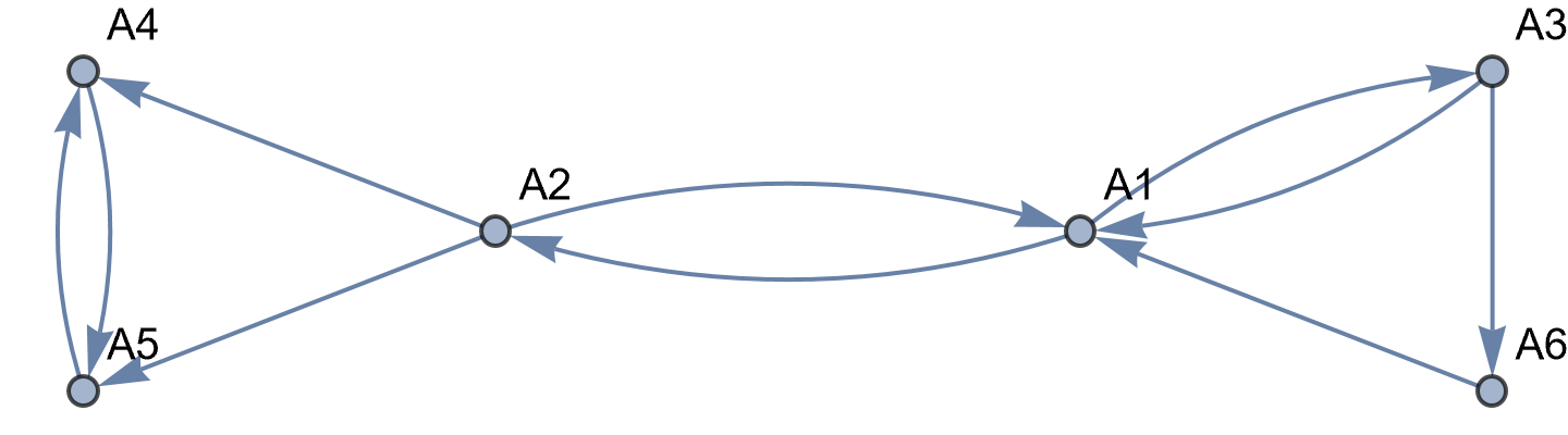
The diagram indicates how six web pages are connected by hyperlinks. For example,
the single directional arrow from A3 to A6 indicates there is a hyperlink on page A3 that
takes the user to page A6 . The two arrows between A4 and A5 indicates
that there is a hyperlink on page A4 to page A5 and a hyperlink on page A5 to
A4.
Below is the matrix in Table format with headings. Next to it is the related graph. It is useful to think of this construction as follows. The arrows indicate the permitted direction. Conversely, travel against the arrow in the opposite direction is not allowed. If the numeral 1 appears in an intersection this means the probability is 100% that you may travel from the node represented by the vertical heading label to the node represented by the horizontal heading label. So, for example, the 1 in the first row, second column means there is a 100% probability that you may travel from A2 to A1. Any travel between any two nodes with a zero in their intersection means that travel between them is not possible. Try going from A5 to A1 on the graph to prove it to yourself.
Stated differently, the matrix has dimensions 6 x 6, corresponding to the six nodes in the graph. Each row and column corresponds to a node (in the order A1, A2, A3, A4, A5, A6). If there is a link from node i to node j, then the element in the i-th row and j-th column of the matrix is 1; otherwise, it is 0. For example, the first row of the matrix represents links from A1 to other pages. The 2nd and 3rd elements in this row are 1, indicating that there are links from A1 to A2 and A3. The rest of the elements in this row are 0, indicating no links from A1 to the other pages.
The diagonal elements of the matrix are all 0, indicating that there is a link only back to itself and that there are no links from any other page to itself.
Mathematica considers this a Sparse Array. See Wolfram Documentation for details.
The adjacency matrix A for this graph represents the network by putting a 1 in the (i, j)-th entry of
A if webpage Ai has a hyperlink to page Aj. For our graph,
Webpage A₁ links to itself, A₂ and A₃
- Web page A₂ links to A₄ and A₅
- Web page A₃ links back to A₁ and to A₆
- Web page A₄ has a two-way link with A₅
- Web page A₅ has no additional links
- Web page A₆ links back to A₁.
For instance, because of the connection from A₃ to
A₆, we get [A]3,6 = 1. Since A₆ does not have a hyperlink to A₃, we have that [A]6,3 = 0. And so on. We build this matrix into Mathematica:
A = {{0,1,1,0,0,0},
{1,0,0,1,1,0},
{1,0,0,0,0,1},
{0,0,0,0,1,0},
{0,0,0,1,0,0},
{1,0,0,0,0,0}}
Then we ask Mathematica to determine some of this matrix powers:
If a square matrix A is invertible, we can also define its negative powers A−n for any positive integer n. Therefore, we can define a meromorphic function for such square matrix. For instance, let
where p(λ) = 𝑎₀ + 𝑎₁λ + ⋯ + 𝑎mλm and q(μ) = b₁μ + b₂μ² + ⋯ + bnμn.
Then for an invertible square matrix A, the following matrix function is well-defined:
Hadamard multiplication is probably what
you would have answered if someone asked you to guess what it
means to multiply two matrices.
For two matrices A and B of the same dimension m × n, the Hadamard product, A ⊙ B, is a matrix of the same dimension as the operands, with elements given by
\[
\left( {\bf A} \odot {\bf B} \right)_{ij} = \left( {\bf A} \right)_{ij} \left( {\bf B} \right)_{ij} .
\]
For example, the Hadamard product of two vectors from 𝔽n is
The concept and notation is the same for matrices as for vectors. Hadamard multiplication involves multiplying each element of one
matrix by the corresponding element in the other matrix.
Mathematica uses regular multiplication sign "*" for Hadamard product:
A = {{1, 2}, {3, 4}}; B = {{-1, 2}, { -2, 3}};
A*B
Element-wise matrix multiplication in computer applications facilitates convenient and efficient coding (e.g., to avoid
using for-loops), as opposed to utilizing some special mathematical properties of Hadamard multiplication. That said, Hadamard
multiplication does have applications in linear algebra. For example, it is key to one of the algorithms for computing the matrix
inverse.
⊙ ⊙
Example 18:
First, we generate ramdomly two 3 × 3 matrices:
For a given m × n matrix A, its
transpose is the n × m matrix, denoted either by \( {\bf A}^T \) or
by At or just by \( {\bf A}' , \) whose entries are formed by interchanging the rows with
the columns; that is, \( \left( {\bf A} \right)_{i,j} = \left( {\bf A}' \right)_{j,i} . \)
When matrix A is considered as an operator, its transposed is usually denoted by prime, A′. However, in linear algebra, transposed matrix is identitied with letter "T."
If A is a square matrix, then its trace is \( \mbox{tr}\left( {\bf A}^{\mathrm T} \right)
= \mbox{tr}\left( {\bf A} \right) ; \)
If A is a square nonsingular matrix, then \( \left( {\bf A}^{\mathrm T} \right)^{-1}
= \left( {\bf A}^{-1} \right)^{\mathrm T} ; \)
If A is a square matrix, then \( \det\left( {\bf A}^{\mathrm T} \right)
= \det\left( {\bf A} \right) . \)
This identity follows immediately from the definition.
It follows from the definition.
It follows from the definition.
Suppose that A = [𝑎i,j]m×n and B = [bi,j]n×p. Then (A B)′ and B′A′ are each of size p × m. Since
\[
\left[ \mathbf{B}' \mathbf{A}' \right]_{i,j} = \sum_{k=1}^n b_{k, i} a_{j,k} = \sum_{k=1}^n a_{j,k} b_{k,i} = \left[ {\bf A}\,{\bf B} \right]_{i,j}
\]
we deduce that (A B)′ = B′A′.
If A is a square matrix, then \( \mbox{tr}\left( {\bf A}^{\mathrm T} \right)
= \mbox{tr}\left( {\bf A} \right) . \)
If A is a square nonsingular matrix, then \( \left( {\bf A}^{\mathrm T} \right)^{-1}
= \left( {\bf A}^{-1} \right)^{\mathrm T} . \)
If A is a square matrix, then \( \det\left( {\bf A}^{\mathrm T} \right)
= \det\left( {\bf A} \right) . \)
Here is a list of basic matrix manipulations with Mathematica:
Example 20: Let us consider the 3-by-4 matrix
First we generate 3-by-4 matrix:
Clear[A, B, subA, subB, matA, matB];
A = Range@12~Partition~4
B = Range[13, 24]~Partition~4
For an m × n matrix A ∈ ℂm×n, its adjoint or the conjugate transpose, also known as the Hermitian transpose, is the n × m matrix, denoted by A✶ obtained by transposing A and applying complex conjugation to each entry (the complex conjugate of 𝑎 + jb being 𝑎 − jb, for real numbers 𝑎 and b).
Theorem 7: Let A and B denote matrices whose sizes are appropriate for the following operations.
Clear[A, B, s];
A = {{8, I , 3 - I, -2 }, {-I, I + 1, 2, 1 - I}, {4*I + 1, I, -1,
2 + I}};
B = {{5, I, 4 - I, -3}, {-I, I + 2, 3, 1 - I}, {5*I + 2, I, -4,
23 + I}};
s = 1 + 2 I
part (a)
ConjugateTranspose[A]
{{8, I, 1 - 4 I}, {-I, 1 - I, -I}, {3 + I, 2, -1}, {-2, 1 + I, 2 - I}}
A == (A\[ConjugateTranspose])\[ConjugateTranspose]
As you see, Mathematica cannot handle this pair of commands. The issue here is due to the nature of scalar multiplication because command ConjugateTranspose is applicable only to matrices. Therefore, we, modify slightly the input:
Calculate the following matrix/vector products by expanding them as a linear
combination of the
of the matrix.
\[
{\bf (a)\ \ \ } \begin{bmatrix} \phantom{-}3&2&1 \\ -1 & e & 2 \end{bmatrix} \begin{bmatrix} 1 \\ -1 \\ 2 \end{bmatrix} , \qquad {\bf (b)\ \ \ } \begin{bmatrix} 2&-3&1 \\ 3&-1&5 \end{bmatrix} \begin{bmatrix} 3 \\ 1 \\ -2 \end{bmatrix}
\]
Prove the following theorem.
Theorem:
If A and B are m x n matrices then, for any scalars λ and μ.
λ(A + B) = λA + λB;
(λ + μ)A = λA + μA;
(−1)A = −A;
λ(μA = (λμ)A = (μλ)A;
0A = 0m×n.
Axier, S., Linear Algebra Done Right. Undergraduate Texts in Mathematics (3rd ed.). Springer. 2015, ISBN 978-3-319-11079-0.